Radial Wavefunctions

Hydrogenic radial wavefunctions are the radial factors in the exact bound states of the attractive point-Coulomb problem. They are where the Bohr scale, exponential decay, near-origin angular-momentum behavior, generalized Laguerre polynomials, radial probability density, and node counting all meet.

The full hydrogen solution is introduced in Hydrogen Atom. This page is the reference home for the radial functions themselves.

Setup and Notation

For a hydrogenic one-electron Coulomb problem, write

$$\psi_{n\ell m}(r,\theta,\phi) = R_{n\ell}(r)Y_\ell^m(\theta,\phi).$$

The angular part is a spherical harmonic. The radial length scale is

$$a = \frac{4\pi\epsilon_0\hbar^2}{\mu Ze^2},$$

where $Z=1$ for hydrogen and $\mu$ is the reduced mass. For hydrogenic ions, $a=a_Z$ in the notation of Hydrogenic Ions.

Define the dimensionless radial variable

$$\rho = \frac{2r}{na}.$$

The allowed quantum numbers are

$$n=1,2,\ldots, \qquad \ell=0,1,\ldots,n-1, \qquad m=-\ell,\ldots,\ell.$$

General Formula

With the standard angular normalization

$$\int_{S^2} \lvert Y_\ell^m\rvert^2\,d\Omega =1,$$

the normalized hydrogenic radial wavefunction is

$$R_{n\ell}(r) = \sqrt{ \left( \frac{2}{na} \right)^3 \frac{(n-\ell-1)!}{2n[(n+\ell)!]} } e^{-\rho/2} \rho^\ell L_{n-\ell-1}^{(2\ell+1)}(\rho).$$

Here $L_{n-\ell-1}^{(2\ell+1)}$ is a generalized Laguerre polynomial. The polynomial degree is

$$n_r=n-\ell-1.$$

This integer is the radial node number. The same integer appears in the relation

$$n=n_r+\ell+1.$$

The factors in $R_{n\ell}$ have distinct jobs:

• $e^{-\rho/2}$ gives the large-radius exponential tail;
• $\rho^\ell$ gives the regular near-origin behavior $R_{n\ell}\sim r^\ell$;
• $L_{n-\ell-1}^{(2\ell+1)}(\rho)$ supplies the radial nodes;
• the prefactor enforces the radial normalization convention.

Normalization and Reduced Function

The radial function $R_{n\ell}$ is normalized with the three-dimensional radial measure:

$$\int_0^\infty \lvert R_{n\ell}(r)\rvert^2r^2\,dr =1.$$

The reduced radial wavefunction is

$$u_{n\ell}(r)=rR_{n\ell}(r).$$

It is normalized with ordinary half-line measure:

$$\int_0^\infty \lvert u_{n\ell}(r)\rvert^2\,dr =1.$$

The boundary condition at the origin for ordinary hydrogenic bound states is

$$u_{n\ell}(0)=0.$$

The detailed endpoint logic is in Boundary Conditions for Radial Wavefunctions.

Low-Lying Examples

For the same length scale $a$, the first few normalized radial functions are:

State	Radial wavefunction
$1s$	$R_{10}(r)=2a^{-3/2}e^{-r/a}$
$2s$	$R_{20}(r)=\frac{1}{2\sqrt2}a^{-3/2}\left(2-\frac{r}{a}\right)e^{-r/(2a)}$
$2p$	$R_{21}(r)=\frac{1}{2\sqrt6}a^{-3/2}\frac{r}{a}e^{-r/(2a)}$

The spectroscopic letters mean

$$s:\ell=0, \qquad p:\ell=1, \qquad d:\ell=2, \qquad f:\ell=3.$$

The radial function alone does not specify the full orbital. The angular factor $Y_\ell^m$ still carries the $m$ dependence and angular nodal structure.

Radial Probability Density

After integrating over angles, the probability of finding the electron between $r$ and $r+dr$ is

$$P_{n\ell}(r)\,dr = \lvert R_{n\ell}(r)\rvert^2r^2\,dr = \lvert u_{n\ell}(r)\rvert^2\,dr.$$

Thus

$$P_{n\ell}(r) = r^2\lvert R_{n\ell}(r)\rvert^2.$$

The factor $r^2$ is not optional. It is why the hydrogen ground-state wavefunction is largest at the origin while its radial probability density is maximal at $r=a$.

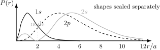
Representative shapes of the radial probability density $P_{n\ell}(r)=r^2\lvert R_{n\ell}(r)\rvert^2$ for $1s$, $2s$, and $2p$ states. The curves are scaled separately to compare shapes; the $2s$ radial node occurs at $r=2a$.

Radial Nodes

Radial nodes are zeros of $R_{n\ell}(r)$, or equivalently of $u_{n\ell}(r)$, in the open interval

$$0\lt r\lt \infty.$$

For hydrogenic bound states, the number of radial nodes is

$$n_r=n-\ell-1.$$

Examples:

State	$n_r$	Comment
$1s$	$0$	no radial node
$2s$	$1$	one radial node at $r=2a$
$2p$	$0$	no radial node, but angular nodes may occur
$3d$	$0$	no radial node because $\ell=n-1$

The endpoint $r=0$ is not counted as a radial node. For $\ell\gt 0$, $R_{n\ell}(0)=0$ because of the regular near-origin factor $r^\ell$, but radial nodes are interior zeros associated with the Laguerre polynomial.

Expectation Values

For fixed $\ell$, radial eigenfunctions with distinct principal quantum numbers are orthonormal:

$$\int_0^\infty r^2 R_{n\ell}^*(r)R_{n'\ell}(r)\,dr =\delta_{nn'}.$$

Different $\ell$ values are not generally orthogonal under this radial integral alone; orthogonality of the full states then comes from the spherical harmonics. For a scalar radial operator $f(r)$,

$$\langle n'\ell'm'\rvert f(r)\lvert n\ell m\rangle =\delta_{\ell'\ell}\delta_{m'm} \int_0^\infty r^2R_{n'\ell}^*(r)f(r)R_{n\ell}(r)\,dr.$$

For a dipole operator the angular selection rules must instead be kept, and the radial factor contains an additional power of $r$:

$$\mathcal R_{n'\ell',n\ell} =\int_0^\infty r^3 R_{n'\ell'}^*(r)R_{n\ell}(r)\,dr.$$

Many hydrogenic radial expectation values can be evaluated exactly. With the length scale $a$ defined above,

$$\langle r\rangle_{n\ell} = \frac{a}{2} \left[ 3n^2-\ell(\ell+1) \right].$$

The mean inverse radius is especially simple:

$$\left\langle \frac{1}{r}\right\rangle_n = \frac{1}{an^2}.$$

Another useful inverse moment is

$$\left\langle\frac{1}{r^2}\right\rangle_{n\ell} =\frac{1}{a^2n^3(\ell+1/2)}.$$

The mean-square radius is

$$\langle r^2\rangle_{n\ell} = \frac{a^2n^2}{2} \left[ 5n^2+1-3\ell(\ell+1) \right].$$

These expectation values scale with $a$ in the obvious way. Hydrogenic ions with larger $Z$ have smaller radii because $a\approx a_0/Z$ for heavy nuclei.

Scaling Across Hydrogenic Ions

For a one-electron ion, the same dimensionless radial functions apply after replacing $a$ by

$$a_Z = \frac{4\pi\epsilon_0\hbar^2}{\mu_ZZe^2}.$$

Thus every radial length, including node positions, maxima, and expectation values of $r$, scales with $a_Z$. Expectation values of $1/r$ scale as $1/a_Z$.

This is the radial-function version of the energy scaling described in Hydrogenic Ions. The shapes are universal in $\rho$; physical units carry the $Z$ and reduced-mass dependence.

Common Mistakes

• Normalizing $R_{n\ell}$ with $dr$ instead of $r^2\,dr$.
• Confusing $R_{n\ell}(r)$ with the radial probability density $P_{n\ell}(r)$.
• Counting $r=0$ as a radial node.
• Forgetting that $2p$ has no radial node even though its angular function has angular nodes.
• Using $a_0$ for every ion instead of the appropriate reduced-mass, charge-$Z$ scale $a_Z$.
• Treating the superscript in $L_{n-\ell-1}^{(2\ell+1)}$ as an exponent rather than a generalized-Laguerre parameter.
• Forgetting that real orbital pictures require angular functions or linear combinations of them, not the radial function alone.

Where This Is Used

• Hydrogen Atom uses these radial functions in the exact bound-state wavefunctions.
• Hydrogenic Ions rescales the same radial functions with $a_Z$.
• Atomic Orbitals combines these radial functions with spherical harmonics to explain $s,p,d,\ldots$ orbitals and their node structure.
• Laguerre Polynomials gives the special-function definitions and identities behind the polynomial factor.
• Spherical Harmonics supplies the angular functions paired with $R_{n\ell}$.
• Normalization Conventions explains why $R$ and $u=rR$ use different radial measures.
• Degeneracy of the Hydrogen Atom uses $n=n_r+\ell+1$ to explain the ideal Coulomb degeneracy.

References

• D. J. Griffiths and D. F. Schroeter, Introduction to Quantum Mechanics, 3rd ed., Cambridge University Press, 2018.
• R. Shankar, Principles of Quantum Mechanics, 2nd ed., Springer, 1994.
• C. Cohen-Tannoudji, B. Diu, and F. Laloë, Quantum Mechanics, Wiley, 1977.
• L. D. Landau and E. M. Lifshitz, Quantum Mechanics: Non-Relativistic Theory, 3rd ed., Pergamon, 1977.
• NIST Digital Library of Mathematical Functions, Chapter 18, Orthogonal Polynomials.

Exercises

1. Use the general formula to recover the $1s$ radial wavefunction.

Solution

For $n=1$ and $\ell=0$,

$$\rho=\frac{2r}{a}, \qquad L_0^{(1)}(\rho)=1.$$

The normalization prefactor becomes

$$\sqrt{ \left( \frac{2}{a} \right)^3 \frac{0!}{2(1)(1!)} } = 2a^{-3/2}.$$

Since $e^{-\rho/2}=e^{-r/a}$, the result is

$$R_{10}(r)=2a^{-3/2}e^{-r/a}.$$

2. Show that the $2s$ radial node occurs at $r=2a$.

Solution

The $2s$ radial function is

$$R_{20}(r) = \frac{1}{2\sqrt2}a^{-3/2} \left( 2-\frac{r}{a} \right) e^{-r/(2a)}.$$

The exponential factor never vanishes. The node is therefore set by

$$2-\frac{r}{a}=0,$$

so

$$r=2a.$$

3. Compute $\langle r\rangle$ for the $1s$ and $2p$ states.

Solution

Use

$$\langle r\rangle_{n\ell} = \frac{a}{2} \left[ 3n^2-\ell(\ell+1) \right].$$

For $1s$, $n=1$ and $\ell=0$, so

$$\langle r\rangle_{10} = \frac{a}{2}(3) = \frac{3a}{2}.$$

For $2p$, $n=2$ and $\ell=1$, so

$$\langle r\rangle_{21} = \frac{a}{2} \left[ 12-2 \right] = 5a.$$

4. For fixed $n=4$, list the allowed $\ell$ values and the corresponding radial node counts.

Solution

For $n=4$,

$$\ell=0,1,2,3.$$

The radial node number is

$$n_r=n-\ell-1.$$

Thus

$$\begin{array}{c c} \ell & n_r \\ \hline 0 & 3 \\ 1 & 2 \\ 2 & 1 \\ 3 & 0 \end{array}$$

Higher $\ell$ at fixed $n$ means fewer radial nodes.

5. Locate the most probable radius of the $1s$ state and explain why it is not the point where the local three-dimensional density is largest.

Solution

The angle-integrated shell density is

$$P_{10}(r)=\frac{4r^2}{a^3}e^{-2r/a}.$$

Away from the endpoint, its logarithmic derivative is

$$\frac{d}{dr}\log P_{10}(r)=\frac{2}{r}-\frac{2}{a},$$

so the interior maximum is at $r=a$. By contrast, $\lvert\psi_{100}(\mathbf r)\rvert^2\propto e^{-2r/a}$ is largest at the origin. The shell probability includes the available volume $4\pi r^2dr$; the local density does not.