Quantum Error Correction and Fault Tolerance

Quantum error correction is a cross-layer discipline. An encoded subspace can satisfy an exact correctability theorem while its syndrome circuit spreads faults; an experiment can show lower logical failure at two finite sizes while saying nothing asymptotic; and a threshold proof can be valid although no available device satisfies its noise assumptions or resource demands. A useful claim must therefore identify the protected task, physical carriers, code, faults, extraction circuit, decoder, logical operations, evidence, and total cost together.

This guide supplies that protection-to-evidence record. Given a memory, logical-operation, scaling, or resource claim, it helps a reader decide whether the licensed output is a correctability certificate, a finite logical channel result, a fault-tolerant operation certificate, a finite suppression or break-even result, a conditional threshold or scaling theorem, or an architecture-specific resource estimate. Those outputs form an evidence-dependency graph rather than a total ranking. Finite evidence does not become an asymptotic theorem by improving, and an asymptotic theorem does not establish that a finite machine meets its premises.

Freeze interfaces before comparing numbers. A decoder needs its detector model and prior; a logical rate needs its denominator, selection, rounds, and output; a resource count needs factories, routing, reaction time, discarded runs, and failure allocation. Nielsen and Chuang (2010) and Lidar and Brun (2013) develop the foundations, while Terhal (2015) reviews quantum-memory assumptions and architectures. Preskill’s Chapter 7 is a useful pre-publication working draft updated in March 2026; detailed fault-tolerant protocols are deferred to its future Chapter 8.

Required background. Circuit Model supplies preparation, gates, measurement, feedforward, circuit locations, and logical resource currencies. Noise in Quantum Information supplies mechanism, fault, context, correlation, leakage, and diagnostic discipline.

Helpful background. Bits, Qubits, Qudits, and Modes separates carriers, states, code subspaces, devices, and logical encodings. Pauli Matrices supplies the matrix and commutation conventions used in finite examples.

Quantum Protection as a Layered Contract

Protect a task, not an abstract word

“Protect the qubit” is not yet a technical request. The intended object may be an unknown state stored for a duration, a classical eigenvalue encoded in a basis state, a logical Bell pair, a repeated parity measurement, a Clifford circuit, a non-Clifford gate, or an entire algorithm with an accepted output rule. These tasks expose different failure modes and require different evidence. A protocol that preserves computational-basis populations can destroy phase coherence; a memory experiment can omit the correlated faults introduced by logical gates; and a postselected demonstration can have a favorable conditional error while consuming an unacceptable number of physical attempts.

Begin by stating the output judged and the trusted boundary. If the output is a logical bit, identify how raw measurements and decoder output become that bit. If it is a logical channel, state the input ensemble or norm in which closeness is assessed. If it is a computation, include state preparation, logical operations, measurements, feedforward, routing, waits, and any repeated factory attempts. The trusted boundary should say whether initialization, classical processing, calibration, and final readout are inside the claim. A theorem about an ideal recovery map does not silently certify the noisy circuit that estimates a syndrome and implements that map.

The physical boundary matters just as much. A “qubit” may be a retained subspace of a multilevel circuit, a spin manifold, a photon with loss sectors, or a logical degree of freedom in an oscillator. Leakage and loss cannot be erased from the model merely because a code is described with Pauli operators. A flagged erasure, an unflagged loss, and coherent leakage followed by return generate different detector records and decoder obligations. The declaration must also name correlated contexts, time dependence, and common-cause processes that can defeat a nominally local fault model.

What this guide owns

This guide owns a twelve-field declaration, a non-total claim-class router, and the dependency logic between correctability, execution, finite evidence, scaling, and resources. It asks whether each layer supplies the inputs required by the next and whether the resulting conclusion stays inside its stated domain. It does not prove the Knill–Laflamme theorem, construct an individual stabilizer or bosonic code, derive a decoder, design a gate gadget, prove a threshold, reproduce a dated experiment, or implement a resource estimator. Those derivations remain with the specialist owners named in the chapter map.

The dependency logic bars several tempting shortcuts. Knill–Laflamme correctability does not imply that a noisy extraction circuit is fault tolerant. A syndrome generally labels an equivalence class, not one unique physical fault. A code-capacity threshold is not a circuit-level threshold. One favorable logical-error point, or even a finite crossing, is not an asymptotic theorem. Memory break-even does not establish universal protected computation. A measured physical fidelity is not automatically the local stochastic, independent, Markovian, or bounded-strength hypothesis of a proof. A logical-qubit count without cycles, factories, routing, classical work, and failure allocation is not an end-to-end resource estimate.

The figure records these allowed and forbidden transitions. There is no finite-suppression-to-threshold edge: finite evidence can test a model or motivate a conjecture, but it does not supply missing asymptotic quantifiers. Resource projection draws on a frozen workload and architecture; a resource estimate is not epistemically above a threshold theorem or finite experiment.

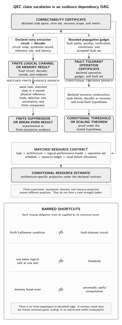
A protection claim escalates only through declared interfaces. Correctability plus a noisy extraction circuit and decoder supports a finite logical channel; bounded fault propagation supports an operation certificate; recursive construction and explicit local-fault hypotheses support a conditional threshold theorem. Matched finite evidence and architecture-specific resource accounting remain separate branches. In particular, Knill–Laflamme does not certify a fault-tolerant circuit, one lower logical rate does not prove a threshold, and memory break-even does not imply useful universal computation.

The Twelve-Field QEC Claim Record

Record fields in declared order

Every worked claim should fill the following record before the result is interpreted. A justified N/A is acceptable when a field truly does not apply. “Unknown,” “not measured,” “assumed stationary,” and “excluded from the trusted boundary” are substantive declarations and must not be replaced by N/A.

Record field	Required declaration
1. Protected task, output, and trusted boundary	State what information or operation is protected, what output is judged, and what lies outside the model.
2. Physical carriers or modes	State retained sectors, leakage or loss sectors, and the physical module boundary.
3. Logical or gauge subspace	State the encoding, projector, code parameters, and any gauge degrees of freedom.
4. Checks and logical operators	State stabilizers or checks, logical operators, and the distance convention.
5. Correctability and faults	State the correctable set, physical fault model, and exact or approximate criterion.
6. Syndrome or detector extraction	State the circuit, ancillas, cadence, reset, measurement record, and detector convention.
7. Decoder and recovery	State the prior, decoder output, recovery or frame rule, latency, and failure policy.
8. Logical operations	State the gadgets, propagation constraints, feedforward, and universal-completion route.
9. Architecture and scaling	State the code family, variants, locality, construction, and scaling and noise hypotheses.
10. Performance evidence	State the estimand, denominator, comparator, data, selection rule, and uncertainty.
11. Resource and failure ledger	State physical qubits or modes, cycles, attempts, classical work, routing, factories, and total-failure allocation.
12. Claim class and owner	State the licensed claim, validity domain, limitations, and canonical next owner.

Fields one through five define what protection would mean. Fields six through eight define the executable protocol. Fields nine through eleven define how the result is scaled, tested, and paid for. Field twelve prevents a local result from migrating into a different claim class. Completing only the code-theory fields can support a correctability certificate, but it cannot support a statement about a running logical memory. Completing only a hardware benchmark can quantify an observed logical channel, but it cannot establish the existence or assumptions of an infinite-family threshold theorem.

Three certificates: protection, execution, evidence

A protection certificate states that a code and recovery satisfy an exact or approximate correctability condition for a declared error set and retained metric. An execution certificate states that specified noisy extraction and logical-operation circuits contain allowed faults so that the decoder or recovery receives a correctable output class. An evidence certificate states what a finite experiment estimates, with denominator, comparator, uncertainty, selection, and resource boundary. Threshold and resource claims add still different quantifiers. None of these certificates is a synonym for “QEC works.”

The claim-class router below is deliberately non-total. A fault-tolerant operation certificate and a finite logical-channel estimate answer different questions; either may exist without the other. A threshold theorem can precede any device implementation, while a device can demonstrate finite suppression under conditions that do not match a published theorem. A resource projection combines conditional models and may be more decision-relevant than either, but it is not thereby stronger evidence.

Claim class	Minimum declared object	Required hypotheses	Required evidence	Does not imply
Detection or filtering	event, flag, acceptance rule, denominator	detector and selection model	flagged and unflagged counts with uncertainty	correction of an unknown logical state
Exact or approximate QEC	code projector, error set, recovery metric	retained Hilbert space and channel or operator span	theorem check or bounded recovery metric	a noisy fault-tolerant circuit
Finite logical memory or channel	complete encoded experiment	extraction, decoder, rounds, selection, reference	logical-channel or failure estimate with uncertainty	an asymptotic threshold
Fault-tolerant logical operation	encoded gadget and allowed faults	bounded propagation and correctable output classes	gadget proof or finite circuit evidence in scope	universal completion or below-threshold operation
Finite suppression or break-even	matched code sizes or named physical reference	fixed task, circuit, decoder, denominator, budget	finite effect and uncertainty; break-even also needs the named reference	a threshold theorem or useful processor
Below-threshold scaling	a declared family and increasing size	matched fault model, decoder, schedule, and fit domain	finite-size scaling with uncertainty and alternatives	a universal threshold value
Threshold theorem	infinite family, gadgets, decoder or recovery, noise class	exact locality, independence or correlation, and metric quantifiers	proof under the stated model	that a device satisfies the hypotheses
Resource projection	logical workload, architecture, error allocation	code, factories, routing, timing, and physical parameters	reproducible ledger and sensitivity analysis	feasibility, availability, or achieved performance

Correctability Before Code Names

Exact correctability and its hypotheses

Let $V:\mathcal H_L\rightarrow\mathcal H_P$ encode a logical Hilbert space into the physical space, and let $P=VV^\dagger$ project onto the code. For a declared operator set $\{E_a\}$, exact subspace correction is characterized by the Knill–Laflamme condition

$$P E_a^\dagger E_b P = c_{ab}P.$$

The Hermitian positive-semidefinite coefficient matrix $C=(c_{ab})$ is independent of the encoded state. Therefore the environment or syndrome degrees of freedom may learn which correctable error sector occurred without learning the logical amplitudes. Knill and Laflamme (1997) prove the criterion and its recovery implications; this guide uses it only as the protection-layer input.

The hypotheses must be stated. The projector identifies the retained code subspace; the operator span specifies what “errors” means; and exact equality selects a strong criterion. If the physical channel has Kraus operators in the span, linearity extends correction to their mixtures and coherent combinations. That statement does not mean that all continuous physical noise is corrected, only that the declared channel lies in the corrected span. Nor does the condition prescribe a fault-tolerant circuit for learning the syndrome or applying recovery.

Degeneracy is compatible with the criterion. Distinct physical operators can act identically on the code, so $C$ need not be diagonal in the initially chosen error basis. What matters is that products $E_a^\dagger E_b$ have no state-dependent action within the logical subspace. Syndrome aliasing across different logical cosets is a different phenomenon: then the observed syndrome does not determine which logical action occurred, and the decoder must choose using a fault model.

Approximate correction and retained metric

Physical noise rarely lies exactly in a finite corrected span, and realistic bosonic codewords can have finite energy rather than ideal support. Approximate QEC therefore asks how closely a recovery $\mathcal R$ makes the encoded noisy channel resemble the identity on logical information. The answer depends on the metric, input scope, and whether a reference system is retained. One possible worst-case channel statement is

$$\frac12\left\| \mathcal R\circ\mathcal N\circ\mathcal V - \mathcal V \right\|_\diamond \le \varepsilon,$$

where $\mathcal V(\rho)=V\rho V^\dagger$. An entanglement-fidelity average, a restricted logical ensemble, and a diamond-norm bound are not interchangeable. A small average error can coexist with a larger worst-case error, and a basis-state success probability does not certify preserved coherence with an external reference.

The approximation also needs a retained physical boundary. Leakage can be included in $\mathcal N$, flagged as an erasure available to recovery, or conditioned away; those choices yield different channels and costs. If a protocol discards runs, report both the conditional logical quality and the acceptance probability. If a recovery depends on analog syndrome information, state whether the metric averages over that record or conditions on it.

Detection, correction, suppression, and mitigation boundaries

Detection distinguishes a flagged event or sector according to an instrument. Correction seeks to restore logical information for a declared fault set. Suppression reports a lower finite error measure under a matched comparison. Mitigation transforms or selects classical outputs without necessarily preserving an unknown quantum state during the computation. These operations can be combined, but the evidence licenses must remain separate.

A detector can be informative without identifying a unique cause. Postselecting on “no flag” can reduce a conditional logical error while lowering yield and changing the retained ensemble. A decoder can use a history of ambiguous detectors to infer a logical coset; its success is statistical and model dependent even when the underlying ideal code corrects a specified fault set. A mitigation transformation applied after logical measurement may improve an expectation but does not retroactively make the encoded gates fault tolerant.

Codes, Checks, Logical Operators, and Distance

Code parameters need a convention

For a qubit subspace code, the notation $[[n,k,d]]$ usually denotes $n$ physical qubits, $k$ logical qubits, and distance $d$ under a declared Pauli-weight convention. A subsystem code may be written $[[n,k,r,d]]$ with $r$ gauge qubits. Those symbols suppress boundary conditions, check weights, geometry, extraction schedule, leakage treatment, and whether distance concerns data errors, phenomenological measurement errors, or a full spacetime circuit. Every use should state enough convention to recover the operational meaning.

The dimension relation for an independent stabilizer group with $n-k$ generators is

$$\dim\mathcal C=2^k,$$

but even this compact statement assumes a qubit Pauli stabilizer subspace with no $-I$ in the stabilizer group. Gauge codes separate measured gauge checks from stabilizers and logical information. Bosonic codes may instead use generalized displacement stabilizers, rotation symmetry, parity structure, or moment conditions. Their resources are modes, excitations, ancillas, and control operations as well as any auxiliary qubits.

Stabilizers, gauge checks, and logical operators

For an abelian stabilizer group $S$ excluding $-I$, the code is the simultaneous $+1$ eigenspace of its elements. Operators in the normalizer $N(S)$ preserve the code; elements outside the phase-extended stabilizer $\langle iI,S\rangle$ act nontrivially on logical information. The quotient $N(S)/\langle iI,S\rangle$ distinguishes a harmless stabilizer or global phase from a logical operator that can share the same measured syndrome as another physical fault. Gottesman (2010) develops the stabilizer, logical-coset, and fault-tolerance language systematically.

Checks are mathematical observables; their implementation is a circuit. An ideal stabilizer relation does not state which ancilla is prepared, how gates are ordered, whether a flag is used, when reset occurs, or how one ancilla fault propagates. In subsystem codes, low-weight gauge checks can be measured and combined to infer stabilizers, introducing temporal and gauge-processing conventions. In oscillator codes, a modular quadrature or parity measurement can require ancillary nonlinear interactions and can import faults from those controls.

Distance depends on the error model

Under a declared Pauli-weight convention for a stabilizer subspace code, distance can be stated as

$$d=\min_{L\in N(S)\setminus\langle iI,S\rangle}\operatorname{wt}(L).$$

Then arbitrary Pauli errors of weight at most

$$t=\left\lfloor\frac{d-1}{2}\right\rfloor$$

are correctable in the ideal bounded-weight model. The conclusion follows because products of two such errors have weight at most $2t<d$ and therefore cannot differ by a nontrivial logical operator while sharing a syndrome. It does not establish a stochastic logical failure probability, a noisy-check threshold, or protection against every error with small amplitude.

The three-bit repetition code illustrates why the convention must be named. As a classical repetition code, or as the quantum bit-flip subcode under $X$ faults, it has $X$-error distance three and corrects one $X$ fault. As a quantum code against the full Pauli set, it has distance one because a single $Z$ acts logically. Calling it a general $[[3,1,3]]$ code would therefore be false. The first executable audit uses only the declared $X$-fault model.

Syndromes, Detectors, and Recovery

Syndromes do not identify unique physical faults

A syndrome records commutation with a set of checks or, more generally, the outcome of a syndrome instrument. For a binary parity-check matrix $H$ and binary error vector $e$, the ideal classical relation is $s=He\pmod 2$. Many errors can produce the same $s$. Some differ by a stabilizer and have the same logical effect; others differ by a logical operator and require different recovery choices. Only the former is stabilizer degeneracy. The latter is logical-coset aliasing and makes decoding an inference problem.

For the repetition fixture,

$$H= \begin{pmatrix} 1&1&0\\ 0&1&1 \end{pmatrix}.$$

The faults $100$ and $011$ both yield syndrome $10$, yet their binary difference is $111$, the logical bit flip. A minimum-weight decoder chooses $100$. Under a low iid bit-flip probability that is the more probable explanation, but the syndrome alone did not establish it. With correlations or nonuniform qubit rates, the preferred representative could change.

Repeated circuits produce detector histories

When checks are measured repeatedly, a raw outcome at time $t$ is not generally a detector by itself. With fixed initial and boundary conventions, a binary detector difference can be defined as

$$\delta_{j,t}=m_{j,t}\mathbin{\mathsf{xor}}m_{j,t-1}.$$

At the first and final boundaries, the comparison may instead use a known preparation, a data measurement, or a virtual boundary check. Those conventions determine which fault locations create which detector events. Omitting them changes the decoding graph and can create apparent unmatched events.

A complete extraction record includes ancilla preparation, controlled interactions, ordering, measurement, reset, idles, leakage handling, cadence, and any flags. Measurement faults can flip one raw check result and therefore create a pair of adjacent temporal detector events. Data faults can persist and alter spatial patterns. Correlated circuit faults can create several events. The circuit-to-detector map is part of the code implementation and cannot be inferred from a static stabilizer list alone.

Recovery can be physical or frame tracked

After decoding, a protocol may apply a physical correction, update a Pauli or more general logical frame, choose an interpretation of final measurements, request a retry, or declare failure. A frame update avoids injecting unnecessary physical gates, but it is not free bookkeeping: future non-Clifford operations, basis changes, feedforward, and final readout must consume the frame correctly. A stale or lost frame record becomes a logical fault.

Recovery is defined relative to a coset decision. If the actual fault is $E$ and the chosen correction is $C$, success requires $CE$ to act trivially on the logical subspace, not that $C=E^\dagger$ as a physical operator. This is why a decoder can succeed without locating the unique microscopic fault. It is also why a recovery selected under the wrong prior can produce a logical error even though every measured syndrome bit was accurate.

The historical constructions of Shor (1995) and Steane (1996) established concrete routes to protecting quantum information, but modern recovery is an integrated physical-and-classical process. Measurement bandwidth, decoder latency, queueing, calibration versions, and fallback behavior belong in the protection claim. Ideal recovery maps remain essential theory; an implemented protocol must also show that the map can be approximated without importing more dangerous faults than the code can handle.

Decoding Is Inference Under a Fault Model

Decoder input, prior, output, and loss

A decoder maps a syndrome or detector record, and sometimes analog metadata, to a logical-coset decision or recovery instruction. Formally, if $D$ is the observed record and $L$ a logical fault class, a maximum-a-posteriori rule selects

$$\widehat L(D) = \arg\max_L \Pr(L\mid D).$$

That probability depends on a prior over physical faults, the extraction circuit, leakage and erasure flags, measurement response, missing data, and calibration epoch. A decoder cannot be described fully by its algorithm family alone.

Logical-coset aliasing and recovery choice

The inference target is normally a logical equivalence class, not an exact error chain. For a syndrome $s$, candidate faults can be decomposed into stabilizer-equivalent classes and nontrivial logical cosets. A decoder succeeds when the chosen recovery and actual fault occupy the same logical coset. Summing probabilities over all members of a coset can therefore outperform selecting the single most likely microscopic fault.

The three-bit audit makes aliasing transparent. The same syndrome contains a one-fault and a two-fault representative separated by the logical word. Under stationary independent Bernoulli faults with $p<1/2$, minimum weight is also maximum likelihood for this pair. Under a burst model in which adjacent flips are common, that equivalence can fail. The algebraic syndrome remains correct while the statistical recovery choice changes.

Latency, backlog, and stale calibration

Real-time QEC is a queueing and control problem as well as an inference problem. Let detector records arrive every $\tau_{\mathrm{cycle}}$ and let the decoder require a random service time $T_D$. A mean service time below the cycle duration does not alone prevent backlog; tail latency, batching, communication, and bursts matter. A frame decision needed before an adaptive gate has a hard deadline even if an offline memory analysis could be completed later.

The record should distinguish throughput from reaction time. A parallel decoder may sustain the average event rate while one logical dependency waits too long. Hardware accelerators can reduce latency but introduce finite precision, compilation versions, and deployment constraints. A fallback policy—delay, use a simpler decoder, discard, or proceed with stale information—changes the logical channel and must be included in the benchmark.

Fault-Tolerant Logical Operations

Bounded fault spread is the obligation

An error-correcting code protects against a declared set of data errors. A fault-tolerant gadget must additionally ensure that a small allowed set of faults occurring inside preparation, extraction, recovery, or a logical operation does not spread into an uncorrectable output. The exact obligation depends on the code, gadget decomposition, fault locations, decoder or recovery, and noise model. “Logical gate” names an action on the code space; “fault-tolerant logical gate” adds a propagation certificate for its implementation.

Transversal operations limit direct propagation because each physical component in one block interacts with at most one component in another block. Yet transversality is neither necessary nor sufficient as a universal description. A transversal gate can still suffer correlated environmental faults outside the assumed model, and most codes do not possess a transversal universal gate set. Flag circuits, verified ancillas, pieceable constructions, code deformation, lattice surgery, gauge fixing, and teleportation enforce containment through different spacetime mechanisms.

The certificate should count faults at physical circuit locations, including preparations, measurements, resets, idles, transport, classical control dependencies, and discarded attempts when those are inside the model. It should state which combinations are malignant: a pair of faults can be harmful not merely because two physical errors occur, but because their locations, propagation, and recovery interpretation jointly form a logical event. This location-aware structure is central to the extended-rectangle analysis of Aliferis, Gottesman, and Preskill (2006).

Universal completion and non-Clifford resources

Stabilizer preparations, Clifford transformations, Pauli measurements, and classical feedforward form a powerful fault-tolerant backbone, but they do not provide universal quantum computation. Universal completion requires a non-Clifford resource, such as an injected and distilled magic state, an appropriate code switch or gauge-fixing step, a native non-Clifford logical operation, or another architecture-specific mechanism. The route chosen changes both fault propagation and the dominant resource ledger.

Magic-state protocols transform several noisy resource states into fewer outputs with lower conditional error under assumptions about their input states and correlations. A factory must therefore specify its protocol, input model, acceptance and failure probabilities, output error definition, attempts, footprint, depth, classical decisions, and throughput. An asymptotic distillation polynomial does not by itself describe a physical factory. Correlated inputs can defeat a calculation that assumes independent errors, and a high rejection probability creates backpressure even when accepted outputs are excellent.

Campbell, Terhal, and Vuillot (2017) review routes toward universal fault tolerance across codes and mechanisms. Their publisher’s 2018 Author Correction corrects swapped gates in Figure 2b; the corrected figure, not the original labels, should guide that comparison. This kind of correction is scientifically consequential even when it does not alter the article’s broad taxonomy.

Memory fault tolerance is not computational fault tolerance

A repeated logical memory probes preparation, syndrome extraction, idles, decoding, and final measurement. It can provide strong evidence about temporal protection and can exercise many components needed for computation. It does not automatically test data movement, logical entangling operations, patch deformation, state injection, magic-state factories, adaptive bases, or the correlations introduced by a compiled workload.

Break-even also remains task-specific. A logical memory can outlive its best physical constituent under a declared storage comparison while having a cycle time too slow for the desired algorithm. A logical gate can outperform a chosen physical construction while the total computation remains factory- or routing-limited. A useful universal processor requires an operation set, workload, accuracy target, timing, and resource envelope, not merely a favorable memory ratio.

From Finite Suppression to Threshold Claims

A threshold is a theorem with a model

An accuracy-threshold theorem states that an infinite family of protected simulations can approximate arbitrarily large ideal computations with controlled overhead when a specified physical-noise strength lies below a positive constant and the theorem’s locality and composition assumptions hold. It quantifies a code or code family, gadget construction, decoder or recovery, noise class, metric, and target simulation error. There is no model-independent percentage called “the threshold.”

A schematic recursion for a code correcting $t$ faults is

$$p_{k+1}\le A p_k^{t+1},$$

where $p_k$ is an effective level-$k$ failure parameter and $A$ summarizes malignant combinations or a suitable bound. This recursion is conditional on the code, gadgets, recovery or decoder, noise class, locality, and metric. The coefficient is not a universal property of distance alone, and a device’s reported average infidelity is not automatically the $p_0$ appearing in the theorem.

Aharonov and Ben-Or (2008) establish fault-tolerant computation under a constant error rate in a rigorous asymptotic setting. Aliferis, Gottesman, and Preskill give a detailed concatenated distance-three analysis. Theorems can treat stochastic local faults, more general local noise in an operator norm, or other models, but their conclusions inherit the exact quantifiers. Independence must not be inserted when a theorem allows bounded correlations, nor omitted when a numerical threshold estimate assumes it.

Pseudothreshold, crossing, and below-threshold scaling

A pseudothreshold is a finite crossing at which a logical error metric for a specified code size and protocol equals a declared physical or lower-level reference. Different sizes, circuit types, decoders, and metrics can have different pseudothresholds. A finite-size crossing is an intersection of estimated logical-performance curves, often used to infer a critical region under a scaling ansatz. Below-threshold scaling is finite evidence that logical error decreases as a declared family grows under matched conditions. None is identical to the asymptotic theorem.

For a simple phenomenological fit over an odd-distance family one might write

$$p_L(d,p) \approx B(p)\left(\frac{p}{p_*}\right)^{(d+1)/2},$$

over a restricted distance and physical-error domain. The parameters depend on circuit, decoder, boundary, schedule, and observable. Corrections to scaling, limited distances, correlated faults, and changing decoder quality can shift an inferred crossing. Fit ranges and alternative models should be prespecified or included in selection uncertainty.

Code-capacity, phenomenological, and circuit-level thresholds answer progressively different fault questions. Code capacity often assumes perfect check information. A phenomenological model adds noisy measurements abstractly. A circuit-level model assigns faults to the extraction circuit and can include propagation and correlated events. A numerical value from one setting cannot be relabeled as another. Likewise, storage and logical-gate thresholds need not coincide.

Finite-size evidence is not an asymptotic theorem

Suppose two sizes yield $\widehat p_5<\widehat p_3$ with a confidence interval for their risk ratio excluding one. That licenses a finite matched suppression claim if the circuit, rounds, decoder, configuration, selection, and denominator are fixed. It does not prove that every larger size improves, that an infinite family has a threshold, or that the observed hardware satisfies a theorem’s noise model. The second audit makes this distinction numerical.

Dated device results should be used as evidence-class examples rather than a leaderboard. Google Quantum AI and Collaborators (2025) report below-threshold surface-code evidence across finite devices under a specific experimental and decoding protocol. The publisher’s 2026 Author Correction corrects only the x-axis and legend labels of Figure 3a, not the logical-error values; claims should follow that corrected scope. Bluvstein and collaborators (2024) demonstrate a logical processor on reconfigurable atom arrays under their stated architecture and experiment. Neither paper supplies a timeless cross-platform ranking.

Code Families and Architecture Choices

Qubit stabilizer and topological routes

Qubit stabilizer codes encode logical degrees of freedom as a common eigenspace of commuting Pauli checks. CSS constructions separate suitable $X$- and $Z$-type checks using classical-code structure; Calderbank and Shor (1996) and Steane’s construction are foundational sources. Concatenated codes recursively encode locations and support classic threshold proofs, while topological codes use spatial locality and extended logical operators.

Surface-code architectures place local checks on a two-dimensional patch and infer spacetime error chains from repeated extraction. Boundaries, check schedules, hook orientation, decoder graph, logical operators, and measurement conventions together define the implementation. Dennis, Kitaev, Landahl, and Preskill (2002) connect topological quantum memory to statistical-mechanical reasoning, while Fowler and collaborators (2012) develop a practical surface-code architecture and overhead perspective.

Quantum LDPC and subsystem routes

Quantum low-density parity-check codes seek sparse checks, often bounded check weight and bounded qubit degree, together with useful rate and distance scaling. Their promise is not captured by asymptotic parameters alone. Check measurement, connectivity, decoder complexity, noisy-syndrome behavior, routing, and fault-tolerant operations determine whether a construction supports an architecture.

Breuckmann and Eberhardt (2021) review the qLDPC landscape as it stood in 2021. Because that review predates the later resolution of the existence of asymptotically good qLDPC families, it must not be cited as evidence that those families exist. It remains valuable for definitions, historical constructions, decoding questions, and the research context available at publication. Current existence or construction claims require their own later primary sources in the specialist page.

Subsystem codes introduce gauge degrees of freedom so that measured gauge operators can be lower weight than the stabilizers they generate. This can simplify extraction or enable gauge fixing, but it adds a layer between raw gauge outcomes, inferred stabilizers, logical state, and decoder. Gauge choices can also interact with logical gates and schedules. Subsystem Codes owns the protected-factor condition, gauge center, bare and dressed logical quotients, gauge-syndrome inference, and Bacon–Shor construction; this guide retains the cross-layer claim router.

Bosonic and concatenated routes

Bosonic codes encode logical information in oscillator modes. They can exploit natural error structure such as photon loss, dephasing, or small phase-space displacements, but finite energy, ancilla faults, leakage outside a modeling truncation, and imperfect control remain part of the channel. Joshi, Noh, and Gao (2021) review bosonic qubits in circuit QED and the physical mechanisms needed to operate them.

Cat codes use coherent-state structure and parity or engineered stabilization; binomial codes use finite Fock superpositions designed around moment and spacing conditions; GKP codes use a phase-space lattice and modular syndrome information. These are related mode encodings, not interchangeable labels. Their energy conventions, syndrome instruments, recoveries, gate mechanisms, and dominant faults differ. The common bosonic owner establishes the family framework, while each substantive leaf owns its construction and evidence.

The task router summarizes first handoffs without duplicating derivations. Owner names are intentionally plain here; the linked chapter map provides the auditable navigation layer.

Goal or constraint	First live owner	Required input	Dominant missing risk	Next owner	Current state
Test correctability	Why Quantum Error Correction Is Possible	encoding and error set	wrong retained space or metric	Stabilizer Formalism or a code leaf	substantive
Represent a stabilizer code	Stabilizer Formalism	Pauli convention and checks	logical-coset or phase error	code-family owner	substantive
Use a two-dimensional local architecture	Surface Code	patch, extraction schedule, and fault model	circuit-level correlations and decoder mismatch	Decoders or Fault-Tolerant Gates	substantive
Explore sparse-check and rate tradeoffs	Quantum LDPC Codes	check family and connectivity	measurement, decoding, and routing overhead	Decoders or Resource Estimation	substantive
Encode in an oscillator	Bosonic Codes	mode, channel, energy, and controls	finite energy, leakage, ancilla faults, and recovery	Cat, Binomial, or GKP Codes	substantive
Infer from syndrome or detector data	Decoders	detector model, prior, latency, and loss	mismatch, backlog, or stale calibration	Logical Benchmarking	substantive
Assess protected computation, scaling, or cost	Fault-Tolerant Gates	workload, code, gadgets, decoder, and budget	theorem, evidence, or architecture mismatch	Threshold Theorem, Resource Estimation, or Logical Benchmarking	substantive

Performance, Break-Even, and Logical Evidence

Define logical failure and denominator

A logical failure is an event defined by the protected task. For a basis-memory experiment it may be a wrong decoded bit after $T$ rounds. For a logical channel it can be a Pauli error class, an entanglement-infidelity estimate, or a worst-case bound. For a gate it includes the intended logical operation and any frame updates. For an algorithm it may be rejection or an output outside an accepted solution set. These estimands cannot be collapsed into one generic logical error rate.

The denominator is equally important. A probability “per round,” “per cycle,” “per shot,” “per logical operation,” and “per unit time” refers to different opportunities. If a run is discarded after a leakage flag or invalid syndrome, report attempted and accepted counts. Conditional failure among accepted runs and unconditional failure per attempt answer different questions. If early stopping changes exposure time, state how the denominator treats shortened runs.

The logical estimand should also preserve basis and task coverage. Reporting the best protected eigenstate can hide a conjugate logical failure. A complete memory-channel claim needs an input ensemble or process-level argument appropriate to the conclusion. A code that detects many faults but discards aggressively may be useful, but its yield and acceptance-conditioned target must stay in the record.

Match the unencoded or constituent reference

“Break-even” requires a named reference. A logical memory can be compared with the best constituent physical qubit, an unencoded physical mode, a repeated physical protocol occupying the same time, or another architecture at matched resources. Each comparator answers a different question. The reference must share the protected task, duration, preparation and measurement scope, success definition, confidence target, and relevant resource boundary.

For an oscillator code, a bare cavity lifetime may not be the correct operational reference if the logical protocol includes ancilla interactions and measurement while the physical reference does not. For a qubit code, comparing one logical round with one physical gate ignores different durations and location counts. For postselection, matching accepted outputs without charging failed attempts can manufacture apparent advantage. State both conditional quality and cost per accepted result.

Sivak and collaborators (2023) report real-time bosonic QEC beyond a declared break-even benchmark. It is a bounded example of a memory-and-control evidence class, not proof of universal computation or a cross-platform ranking. The correct scientific use is to examine its protected task, physical reference, feedback implementation, and uncertainty, then ask whether a new claim matches those conditions.

Carry uncertainty, selection, and decoder version

For $f$ failures in $N$ stationary independent Bernoulli trials, $\widehat p=f/N$ is a point estimate, not a complete result. Wilson intervals avoid some poor small-sample behavior of the elementary Wald interval. Comparisons need an interval or model for a difference or ratio as well as each marginal proportion. The second audit uses Wilson intervals for each proportion and a separately declared approximate independent-binomial log-Wald interval for the risk ratio; it never obtains a ratio interval by dividing Wilson endpoints.

Selection decisions can dominate reported scaling. Code sizes, physical operating points, round ranges, decoder hyperparameters, postselection thresholds, fit windows, and plotted metrics should be frozen or their selection uncertainty carried forward. If data used to train or tune the decoder are also used for the final estimate, the nominal confidence interval does not cover the adaptive procedure. Hold out the final comparison or use a method that explicitly models selection.

Every result should identify decoder version, calibration version, circuit compilation, hardware configuration, and acquisition times. Redecoding historical data with an improved algorithm is scientifically valuable, but it supports an offline counterfactual unless that decoder met the original real-time constraints. Mixing versions without labels can make an apparent trend that is actually a software change.

Resource and Failure-Budget Accounting

Physical qubits or modes, cycles, and classical control

A resource estimate starts from a logical workload, not from a code distance. State logical qubits or modes, operation counts, dependency depth, measurement and feedforward structure, target runtime, and allowed total failure. Then map the workload to code blocks, ancillas, extraction cycles, logical gadgets, routing, and classical processing. Peak footprint, integrated spacetime volume, and wall-clock time are complementary currencies.

For a code of distance $d$, a schematic physical footprint $q(d)$ and logical cycle time $\tau_L(d)$ are not enough. The extraction schedule may use additional ancillas, routing space, reserve patches, calibration structures, and inactive regions. Decoder work can scale with detector volume and must meet reaction-time deadlines. Control bandwidth and measurement-reset cadence can limit parallelism even when enough physical qubits are nominally available.

Mode encodings require a similarly complete ledger. Count oscillator modes, auxiliary nonlinear elements or qubits, average and peak excitation, syndrome ancillas, reset, control pulses, and failed preparations. A statement that one logical qubit occupies one oscillator hides the support hardware and time. Hybrid concatenated schemes must count both inner-code control and outer-code checks, including correlations crossing the interface.

Factories, routing, reaction time, and discarded runs

Non-Clifford resource factories can dominate footprint and throughput. A complete factory model includes protocol levels, input and output error conventions, acceptance probability, correlated-input assumptions, attempts, cycle depth, routing ports, buffers, classical verification, and failure behavior. Average production above average consumption is insufficient if bursty demand and stochastic rejection cause stalls. Buffering reduces stall risk while adding footprint and storage errors.

Reaction time joins quantum and classical resources. Measurement integration, data movement, decoding, frame propagation, control compilation, and actuation all precede some adaptive choices. Parallel throughput does not remove a sequential dependency. If a T gate, teleportation step, or branch must wait, the resulting idles and storage errors feed back into the logical model.

Discarded attempts are resources and evidence. Failed state injection, rejected factory outputs, invalid syndrome records, heralded loss, and postselected logical runs consume hardware time and can bias the retained ensemble. Report acceptance as a probability with uncertainty, the stopping or fixed-budget rule, and the cost distribution rather than only its mean when tails affect deadlines.

Allocate the end-to-end failure budget

Let a workload expose failure events $F_1,\ldots,F_J$ for logical operations, memories, factories, routing, decoding, and final readout. A conservative union bound gives

$$\Pr\!\left(\bigcup_{j=1}^{J}F_j\right) \le \sum_{j=1}^{J}\Pr(F_j),$$

without requiring independence. Allocating $\varepsilon_j$ with $\sum_j\varepsilon_j\le\varepsilon_{\mathrm{tot}}$ is therefore a valid sufficient planning rule when each component bound is valid in the composed process. Dependence and common-cause faults still matter because they can invalidate the component bounds or introduce omitted events.

A product-form success estimate such as $\prod_j(1-p_j)$ invokes independence or an adequately justified conditional factorization. It may sharpen the union bound, but it must not appear by default. Repeated logical operations can share calibration drift, factories can feed correlated states, and a control outage can affect many blocks at once. Scenario and stress analysis should include such common causes.

Two Reproducible Finite Audits

The two fixtures below are deliberately separate. Audit 1 is an exact finite probability calculation for the classical three-bit repetition code, equivalently the quantum bit-flip subcode under iid $X$ faults and perfect checks. Audit 2 is a synthetic matched data fixture. Neither is hardware evidence, and the $p=0.08$ model from Audit 1 must not be used to explain the rates in Audit 2.

Audit 1 — Syndrome ambiguity and decoder dependence

With the declared parity check $H$, faults $100$ and $011$ both produce syndrome $10$ and differ by logical word $111$. This is aliasing across logical cosets, not stabilizer degeneracy. Under a separate toy model of stationary independent Bernoulli $X$ faults with $p=0.08$, their probabilities are $0.067712$ and $0.005888$. Their syndrome probability is $0.0736$. A minimum-weight decoder chooses $100$ and fails conditionally when $011$ occurred, giving conditional logical failure $0.005888/0.0736=0.08$.

The calculation establishes that a syndrome is not a unique physical-fault label and that recovery depends on a prior. It does not describe the full Pauli behavior of a $[[3,1,3]]$ code: the repetition subcode has full Pauli distance one and only the declared $X$-error distance is three. Correlated or nonuniform faults would change the conditional inference while leaving the binary syndrome relation unchanged. The general inference problem belongs to Decoders.

Audit 2 — Finite suppression versus threshold evidence

The synthetic fixture uses independent stationary Bernoulli trials, identical endpoint definitions, and $N_3=N_5=1{,}000{,}000$. The observed failures are $f_3=240$ and $f_5=100$, so $\widehat p_3=0.00024$, $\widehat p_5=0.0001$, and point suppression is $2.4$. The 95% Wilson interval at size three is

$$[0.00021149923236326887,0.00027234036780752547],$$

and at size five it is

$$[0.00008222785989325881,0.00012161281588187336].$$

For the separately declared approximate independent-binomial log-Wald risk-ratio interval, use

$$\operatorname{SE}(\log \widehat R) = \sqrt{ \frac{1-\widehat p_3}{N_3\widehat p_3} + \frac{1-\widehat p_5}{N_5\widehat p_5} }, \qquad \mathrm{CI}_{R} := \exp\!\left[ \log\widehat R \mathbin{\pm} z\operatorname{SE}(\log\widehat R) \right],$$

with $z=1.959963984540054$. The ratio-scale interval has lower endpoint $1.9006631082457575$ and upper endpoint $3.0305212822888263$. It is approximate, is not a Wilson interval, and is not obtained by dividing Wilson endpoints. The fixture licenses finite matched suppression only when circuit, rounds, decoder, configuration, selection, and denominator are frozen. It does not establish break-even without a named physical or unencoded comparator and proves neither a threshold theorem nor useful computation.

// QEC_AND_FAULT_TOLERANCE_FINITE_AUDITS
import assert from 'node:assert/strict';

const close = (actual, expected, tolerance = 1e-12) => {
  assert.ok(
    Math.abs(actual - expected) <= tolerance,
    `expected ${expected}, received ${actual}`,
  );
};

// Audit 1: syndrome ambiguity in a three-bit repetition model.
const parityCheck = [
  [1, 1, 0],
  [0, 1, 1],
];
const xor = (left, right) => left.map((bit, index) => bit ^ right[index]);
const syndrome = (fault) => parityCheck.map((row) =>
  row.reduce((value, bit, index) => value ^ (bit & fault[index]), 0)
);
const hammingWeight = (bits) => bits.reduce((sum, bit) => sum + bit, 0);
const faultProbability = (fault, probability) =>
  fault.reduce(
    (product, bit) => product * (bit ? probability : 1 - probability),
    1,
  );

const fault100 = [1, 0, 0];
const fault011 = [0, 1, 1];
const logicalWord = [1, 1, 1];
const toyFaultProbability = 0.08;
const probability100 = faultProbability(fault100, toyFaultProbability);
const probability011 = faultProbability(fault011, toyFaultProbability);
const syndrome10Probability = probability100 + probability011;
const minimumWeightFailure = probability011 / syndrome10Probability;

assert.deepEqual(syndrome(fault100), [1, 0]);
assert.deepEqual(syndrome(fault011), [1, 0]);
assert.deepEqual(xor(fault100, fault011), logicalWord);
assert.equal(hammingWeight(fault100), 1);
assert.equal(hammingWeight(fault011), 2);
close(probability100, 0.067712);
close(probability011, 0.005888);
close(syndrome10Probability, 0.0736);
close(minimumWeightFailure, 0.08);

// Audit 2: finite matched suppression with declared intervals.
const z = 1.959963984540054;
const wilsonInterval = (failures, trials) => {
  const estimate = failures / trials;
  const zSquared = z ** 2;
  const denominator = 1 + zSquared / trials;
  const center = (estimate + zSquared / (2 * trials)) / denominator;
  const radius = z * Math.sqrt(
    estimate * (1 - estimate) / trials + zSquared / (4 * trials ** 2),
  ) / denominator;
  return [center - radius, center + radius];
};

const trials3 = 1_000_000;
const trials5 = 1_000_000;
const failures3 = 240;
const failures5 = 100;
const estimate3 = failures3 / trials3;
const estimate5 = failures5 / trials5;
const suppression = estimate3 / estimate5;
const interval3 = wilsonInterval(failures3, trials3);
const interval5 = wilsonInterval(failures5, trials5);
const logRiskRatioStandardError = Math.sqrt(
  (1 - estimate3) / (trials3 * estimate3) +
  (1 - estimate5) / (trials5 * estimate5),
);
const riskRatioInterval = [
  Math.exp(Math.log(suppression) - z * logRiskRatioStandardError),
  Math.exp(Math.log(suppression) + z * logRiskRatioStandardError),
];

assert.equal(trials3, trials5);
assert.equal(failures3, 240);
assert.equal(failures5, 100);
close(estimate3, 0.00024);
close(estimate5, 0.0001);
close(suppression, 2.4);
close(interval3[0], 0.00021149923236326887);
close(interval3[1], 0.00027234036780752547);
close(interval5[0], 0.00008222785989325881);
close(interval5[1], 0.00012161281588187336);
close(riskRatioInterval[0], 1.9006631082457575);
close(riskRatioInterval[1], 3.0305212822888263);

console.log('QEC-and-fault-tolerance finite audits: PASS');

Chapter Map and Canonical Owners

Live routes through this chapter

The Quantum Information and Computation root supplies volume context; What Is Quantum Information? supplies first orientation; the Quantum Information Roadmap supplies a staged route; and Math Needed for Quantum Information supplies the algebra, probability, inference, scaling, and accounting prerequisites.

The complete chapter map preserves the planned order. All twenty-five leaf routes are substantive and linked, so each question below leads to an implemented canonical owner rather than a route promise.

Chapter question	Canonical owner	State and exit
Why is correction compatible with no-cloning and measurement disturbance?	Why Quantum Error Correction Is Possible	substantive; exact and approximate correctability
How do Pauli operators prepare the stabilizer language?	Pauli Group and Stabilizers	substantive bridge; phase-safe small-list checks and algebraic error signatures; full formalism remains with Stabilizer Formalism
How are code spaces and Clifford transformations represented?	Stabilizer Formalism	substantive; stabilizer and symplectic algebra
How are checks measured without revealing logical amplitudes?	Syndrome Measurement	substantive; signed check circuits, ordered fault propagation, repeated records, and boundary-aware detectors
What do the repetition-code examples establish?	Three-Qubit Codes	substantive; bit/phase duality, ideal recovery, restricted distance, and targeted-noise failure
What is the smallest perfect qubit code?	Five-Qubit Code	substantive; cyclic [[5,1,3]] code, perfect packing, and full-Pauli correction
How does the Shor construction combine bit- and phase-flip protection?	Shor Code	substantive; concatenated [[9,1,3]] code, twenty-two one-error syndrome classes, and degenerate full-Pauli recovery
How does the Steane code realize a self-dual CSS construction?	Steane Code	substantive; weakly self-dual Hamming-derived [[7,1,3]] CSS code, nondegenerate recovery, and transversal Clifford operations
How are classical codes combined into CSS codes?	CSS Codes	substantive; paired binary checks, nested classical codes, logical quotients, asymmetric distance, and split syndrome algebra
How does local topological protection work on a planar patch?	Surface Code	substantive; geometry, extraction, decoding, and overhead
How do color-code constructions differ?	Color Codes	substantive; 2-colex checks, colored boundaries, logical operators, transversal gates, decoding, and bounded evidence
What is common across topological quantum codes?	Topological Codes	substantive; local checks, homology, defect dictionaries, active versus passive protection, and dimensional limits
What do sparse checks and finite-rate targets change?	Quantum LDPC Codes	substantive; active construction, decoding, and architecture tradeoffs
How do gauge degrees of freedom change extraction and gates?	Subsystem Codes	substantive; protected tensor factors, gauge quotients, inferred stabilizers, Bacon–Shor codes, and bounded tradeoffs
How can an oscillator carry logical redundancy?	Bosonic Codes	substantive; common mode-code framework
How do coherent-state encodings use bias and parity?	Cat Codes	substantive; cat-family construction and evidence
How do finite Fock superpositions match loss moments?	Binomial Codes	substantive; binomial-family construction and evidence
How do phase-space lattices correct small displacements?	GKP Codes	substantive; GKP construction, recovery, and evidence
How is detector data converted into a logical decision?	Decoders	substantive; inference, priors, latency, and evaluation
How are faults prevented from spreading through logical operations?	Fault-Tolerant Gates	substantive; gadget and propagation contracts
How are non-stabilizer resources injected and distilled?	Magic State Distillation	substantive; protocol and factory contracts
How do parity measurements operate between logical patches?	Lattice Surgery	substantive; merge, split, routing, and spacetime evidence
What does a threshold theorem actually quantify?	Threshold Theorem	substantive; theorem assumptions and limitations
How are logical workloads converted into physical resources?	Resource Estimation	substantive; end-to-end ledger and sensitivity
How should finite logical performance be measured?	Logical Benchmarking	substantive; denominators, comparators, uncertainty, and evidence

Canonical owner firewall

The guide routes executable detector and tableau work to Stabilizer Simulation, dated demonstrations and matched experimental records to Error-Correction Case Studies, and contingent architecture comparisons and update triggers to the Fault-Tolerant Quantum Computing Frontier.

The firewall is also a citation rule. A review can orient a landscape but cannot replace a later primary result it predates. A device paper supports the task and evidence it reports, not a current platform ranking. A theorem supports its quantified model, not a hardware translation that has not been shown. When a claim crosses layers, cite and declare each layer rather than stretching one source across the entire chain.

Common QEC and Fault-Tolerance Claim Failures

Treating Knill–Laflamme as a circuit certificate. The condition certifies recoverability for a code and error span. It does not specify a noisy extraction circuit, decoder latency, bounded propagation, or resource cost. Add an execution certificate before making a fault-tolerant-circuit claim.

Treating a syndrome as a unique fault label. Stabilizer-equivalent errors can share a logical action, while different logical cosets can also share a syndrome. State the prior, decoder target, and recovery rule; call cross-coset ambiguity aliasing rather than degeneracy.

Calling the repetition subcode a general distance-three quantum code. The three-bit construction has $X$-error distance three in the declared bit-flip model but full Pauli distance one. Always name the operator set behind distance and the resulting value of $t$.

Replacing a circuit-level model with a code-capacity number. Perfect-syndrome data-error studies omit ancilla, measurement, reset, idle, and propagation faults. Preserve the threshold convention and never compare its number directly with a device metric from another model.

Promoting one lower logical point to a threshold. A finite reduction supports a scoped suppression claim with uncertainty. A threshold theorem requires an infinite family and explicit noise, locality, gadget, decoder, and metric quantifiers; a finite crossing still needs scaling alternatives.

Calling conditional improvement break-even. Break-even needs a named unencoded or physical reference at matched task, time, selection, and cost. Report rejected attempts and unconditional performance as well as the retained result.

Inferring computation from memory. Memory exercises only a subset of logical locations. Universal computation also needs fault-tolerant operations, non-Clifford resources, routing, adaptive control, and an end-to-end workload budget.

Calling one fidelity a theorem premise. Average gate fidelity can hide coherent, correlated, leakage, or context-dependent faults and need not equal the strength used by a proof. Supply a justified metric translation and test the theorem’s physical assumptions.

Counting logical qubits without a resource ledger. Include modes or physical qubits, syndrome ancillas, cycles, factories, routing, buffers, classical throughput and reaction time, failed attempts, calibration, and failure allocation. A projection remains conditional until availability and performance are established.

Exercises

Freeze a Complete QEC Claim

Draft all twelve record fields for a logical memory that runs $100$ extraction rounds and returns one decoded logical bit. Identify at least one trusted-boundary choice that would change the claim.

Solution

Assume a declared code and basis-state memory task. Record the output bit and whether preparation and readout count; physical carriers and leakage sectors; code projector and parameters; checks, logicals, and distance convention; fault model; complete extraction schedule; prior, decoder, frame, and latency; the absence of non-memory gadgets; finite code size; failure per attempted run with comparator and interval; qubits, rounds, discarded runs, and classical work; and the finite-memory claim class. If readout is trusted in one version and included in another, the estimand changes. Correctability, decoding, benchmarking, and resource questions go to their respective owners.

Classify Exact and Approximate Correctability

A recovery has entanglement infidelity below $10^{-4}$ on a stated channel ensemble, but no exact operator-span equality is shown. Classify the result and state what cannot be concluded.

Solution

Assume the ensemble, recovery, retained space, and fidelity convention are frozen. This is an approximate recovery statement for that metric, not an exact Knill–Laflamme certificate and not a worst-case diamond-norm bound. It says nothing by itself about noisy syndrome extraction, bounded fault propagation, threshold scaling, or an implemented device. Route the exact-versus-approximate proof to Why Quantum Error Correction Is Possible, then route circuit and evidence questions separately.

Reproduce Syndrome Ambiguity

Using the stated parity check, verify that $100$ and $011$ have syndrome $10$, differ by $111$, and give conditional failure $0.08$ for the minimum-weight choice under the toy prior.

Solution

Multiply each vector by $H$ modulo two: both yield $(1,0)$. Their xor is $111$, so they lie in different logical classes for the repetition problem. With iid $p=0.08$, their probabilities are $p(1-p)^2=0.067712$ and $(1-p)p^2=0.005888$. The conditional failure is

$$0.005888/(0.067712+0.005888)=0.08.$$

This is logical-coset aliasing under a toy bit-flip prior; Decoders owns the general inference problem.

State a Distance Convention

Explain when $t=\lfloor(d-1)/2\rfloor$ follows and why it cannot be applied to an arbitrary correlated fault model without qualification.

Solution

Assume distance is minimum Pauli weight in the nontrivial logical coset and faults are classified by that same weight. Two errors of weight at most $t$ have a product of weight at most $2t<d$, so they cannot share a syndrome while differing logically; hence they are correctable. A correlated event can have small occurrence order yet high Pauli weight, and an erasure or displacement model uses different structure. Route formal distance proofs to the code and correctability owners and circuit-effective distance to the implementation owner.

Separate Syndrome, Detector History, and Recovery

Describe these three objects for repeated binary check measurements and state one boundary convention.

Solution

Assume raw check outcome $m_{j,t}$. A syndrome is the check information at a specified time; a detector history can use $\delta_{j,t}=m_{j,t}\mathbin{\mathsf{xor}}m_{j,t-1}$ across rounds; recovery is the physical correction, frame update, or final interpretation selected from the history and prior. At the first round, compare with a known prepared check value; at the last, state whether data measurements close the boundary. Extraction details belong to the code implementation, while general inference belongs to Decoders.

Audit Fault Spread and Universality

A transversal logical Clifford is shown to contain one allowed fault per output block. What is certified, and what further declaration is needed for universal computation?

Solution

Assume the code corrects the resulting output class and the physical-fault and location models match the propagation argument. The result is a bounded-fault-spread certificate for that Clifford gadget. It does not certify every logical operation, below-threshold execution, or universal completion. State how a non-Clifford resource is supplied—such as injection and distillation—and audit its correlated inputs, acceptance, factories, feedforward, and failure budget. Fault-Tolerant Gates and Magic State Distillation retain those specialist mechanisms.

Reject a Threshold Overclaim

Reproduce the two Wilson intervals and risk-ratio interval in Audit 2, then write the strongest licensed conclusion.

Solution

Assume independent stationary Bernoulli trials with matched endpoints and no adaptive selection. Wilson’s formula gives the stated marginal intervals. The declared approximate log-Wald ratio is

$$[1.9006631082457575,3.0305212822888263].$$

The result supports finite suppression for those two sizes, circuit, rounds, decoder, configuration, and denominator. It is not break-even without a named physical reference and is not a threshold theorem. Route statistics to Logical Benchmarking and asymptotic quantifiers to Threshold Theorem.

Complete an End-to-End Handoff

Turn a favorable logical-memory result into the next records needed for one protected non-Clifford operation and an architecture resource estimate.

Solution

Freeze the memory’s code, circuit, decoder, estimand, and uncertainty, then add a bounded-propagation record for every location in the logical operation. Declare the non-Clifford supply, factory acceptance and output error, routing, frame reaction time, and fallback policy. Map the workload to qubits or modes, cycles, buffers, classical work, and a union-bound failure allocation with sensitivity scenarios. Include one hardware boundary, such as limited two-dimensional routing or a mode–ancilla interface. Operation, factory, resource, benchmarking, and hardware owners receive separate handoffs.

References

• D. Aharonov and M. Ben-Or, “Fault-tolerant quantum computation with constant error rate,” SIAM Journal on Computing 38, 1207–1282 (2008), doi:10.1137/S0097539799359385.
• P. Aliferis, D. Gottesman, and J. Preskill, “Quantum accuracy threshold for concatenated distance-3 codes,” Quantum Information and Computation 6, 97–165 (2006), doi:10.26421/QIC6.2-1.
• D. Bluvstein et al., “Logical quantum processor based on reconfigurable atom arrays,” Nature 626, 58–65 (2024), doi:10.1038/s41586-023-06927-3.
• N. P. Breuckmann and J. N. Eberhardt, “Quantum Low-Density Parity-Check Codes,” PRX Quantum 2, 040101 (2021), doi:10.1103/PRXQuantum.2.040101.
• A. R. Calderbank and P. W. Shor, “Good quantum error-correcting codes exist,” Physical Review A 54, 1098–1105 (1996), doi:10.1103/PhysRevA.54.1098.
• E. T. Campbell, B. M. Terhal, and C. Vuillot, “Roads towards fault-tolerant universal quantum computation,” Nature 549, 172–179 (2017), doi:10.1038/nature23460; Author Correction, Nature 559, E6 (2018), correcting swapped gates in Figure 2b, doi:10.1038/s41586-018-0116-0.
• E. Dennis, A. Kitaev, A. Landahl, and J. Preskill, “Topological quantum memory,” Journal of Mathematical Physics 43, 4452–4505 (2002), doi:10.1063/1.1499754.
• A. G. Fowler, M. Mariantoni, J. M. Martinis, and A. N. Cleland, “Surface codes: Towards practical large-scale quantum computation,” Physical Review A 86, 032324 (2012), doi:10.1103/PhysRevA.86.032324.
• Google Quantum AI and Collaborators, “Quantum error correction below the surface code threshold,” Nature 638, 920–926 (2025), doi:10.1038/s41586-024-08449-y; Author Correction, Nature 653, E5 (2026), correcting only the x-axis and legend labels in Figure 3a, not the logical-error values, doi:10.1038/s41586-026-10559-8.
• D. Gottesman, “An introduction to quantum error correction and fault-tolerant quantum computation,” in Quantum Information Science and Its Contributions to Mathematics, Proceedings of Symposia in Applied Mathematics 68, 13–58 (2010), doi:10.1090/psapm/068/2762145, arXiv:0904.2557.
• A. Joshi, K. Noh, and Y. Y. Gao, “Quantum information processing with bosonic qubits in circuit QED,” Quantum Science and Technology 6, 033001 (2021), doi:10.1088/2058-9565/abe989.
• E. Knill and R. Laflamme, “Theory of quantum error-correcting codes,” Physical Review A 55, 900–911 (1997), doi:10.1103/PhysRevA.55.900.
• D. A. Lidar and T. A. Brun, eds., Quantum Error Correction, Cambridge University Press (2013), doi:10.1017/CBO9781139034807.
• M. A. Nielsen and I. L. Chuang, Quantum Computation and Quantum Information, 10th anniversary edition, Cambridge University Press (2010), doi:10.1017/CBO9780511976667.
• J. Preskill, Quantum Information, Chapter 7, “Quantum Error Correction,” working draft updated March 2026, pre-publication chapter.
• P. W. Shor, “Scheme for reducing decoherence in quantum computer memory,” Physical Review A 52, R2493–R2496 (1995), doi:10.1103/PhysRevA.52.R2493.
• V. V. Sivak et al., “Real-time quantum error correction beyond break-even,” Nature 616, 50–55 (2023), doi:10.1038/s41586-023-05782-6.
• A. M. Steane, “Error correcting codes in quantum theory,” Physical Review Letters 77, 793–797 (1996), doi:10.1103/PhysRevLett.77.793.
• B. M. Terhal, “Quantum error correction for quantum memories,” Reviews of Modern Physics 87, 307–346 (2015), doi:10.1103/RevModPhys.87.307.