Stabilizer Simulation

Short Definition

Stabilizer simulation is the efficient classical execution of circuits that preserve stabilizer structure: stabilizer-state preparations, Clifford gates, Pauli measurements, resets, and compatible classical feedforward. Instead of storing $2^n$ complex amplitudes for $n$ qubits, a simulator stores polynomial- size Pauli-generator data, graph-state data, or a reference stabilizer state plus Pauli frames.

This page owns implementation choices, requested outputs, repeated-shot sampling, Pauli-frame execution, quantum-error-correction workflows, detector and decoder interfaces, performance accounting, and validation. Stabilizer Formalism remains the canonical home for Pauli groups, binary symplectic algebra, stabilizer codes, logical operators, tableau semantics, Clifford conjugation, measurement updates, and the Gottesman–Knill theorem. Quantum Circuit Simulation owns the general simulation contract and exact state-vector baseline.

The distinction is useful: the formalism proves closure and specifies the mathematical updates; a simulator must choose a data layout, random-branch semantics, compilation strategy, output format, noise interface, and evidence that those updates were implemented correctly.

Why Closure Changes the Cost

A pure stabilizer state is specified by $n$ independent commuting Pauli generators with signs. An augmented Aaronson–Gottesman-style tableau commonly stores $n$ stabilizer rows and $n$ destabilizer rows, each with $2n$ binary Pauli coordinates and phase data. Its raw binary scale is therefore

$$M_{\mathrm{tab}} = O(n^2)\ \mathrm{bits},$$

compared with

$$M_{\mathrm{sv}} = O(2^n)\ \mathrm{complex\ numbers}$$

for a generic state vector. The exact constants depend on representation, alignment, word packing, scratch space, and whether both a tableau and its inverse are retained.

For example, a raw $2n\times(2n+1)$ binary array at $n=1{,}000$ contains about four million bits, or roughly half a mebibyte before overhead. A 1,000-qubit state vector is not merely inconvenient; its $2^{1000}$ amplitudes cannot be stored by any foreseeable classical machine.

The compression works because Clifford evolution maps Pauli constraints to Pauli constraints. It does not mean that the stabilizer state’s full amplitude list is short. A graph state can have support on exponentially many basis states while its generator description remains polynomial.

Polynomial does not mean constant

The classic augmented-tableau algorithm applies a local Clifford gate by updating relevant columns and phases across the rows, giving linear work in $n$ in a straightforward layout. Pauli measurement may require row reduction and can take quadratic work. Alternative representations change these costs. An inverse tableau can make some deterministic measurements linear; graph-state representations can favor circuits whose evolving graph remains sparse; sparse or bit-packed tableaus change constants and sometimes practical scaling.

The correct performance statement therefore names the representation and operation mix. “Stabilizer circuits are efficient” is a complexity-class statement, not a benchmark result for every implementation and every output.

What a Stabilizer Simulator Can Return

The natural outputs are not generic amplitude arrays.

Output	Meaning	Typical cost driver
final tableau or generators	compact final stabilizer description	Clifford updates and canonicalization
one measurement trajectory	sampled outcomes with conditional state updates	number and type of Pauli measurements
many shots	repeated outcome or detector samples	analysis cost, frame propagation, output volume
Pauli expectation	$0$, $+1$, or $-1$ for a pure stabilizer state	membership and sign query
syndrome or detector stream	parity checks derived from measurements	circuit execution and parity transform
logical observable sample	encoded output bit or eigenvalue	logical definition and frame correction
Clifford action	symplectic action plus phase data	circuit compilation or tableau propagation
stabilizer-state overlap	exact structured overlap	elimination or graph operations

For a pure stabilizer state and Hermitian Pauli $P$,

$$\langle P\rangle = \begin{cases} +1, & P\in S,\\ -1, & -P\in S,\\ 0, & P\notin\pm S. \end{cases}$$

This makes Pauli observables especially convenient. A general non-Pauli observable must be decomposed into Pauli terms or handled by another method, and the number of terms may itself be large.

Sampling is efficient even when listing the full output distribution is not. A circuit can have exponentially many possible bitstrings. The simulator produces one trajectory or a requested number of shots without enumerating all outcomes.

The Stabilizer-Circuit Contract

The efficiently closed circuit family includes:

• preparation of stabilizer states such as computational-basis and graph states;
• Clifford gates, commonly generated by $H$, $S$, and CNOT;
• measurement of Hermitian Pauli observables;
• discard and reset implemented within stabilizer operations;
• classical control that selects later stabilizer operations from measurement results.

A measurement result convention must be explicit. This page uses bit $m\in\{0,1\}$ for eigenvalue

$$\lambda_m=(-1)^m.$$

Thus bit 0 means the $+1$ eigenspace and bit 1 means the $-1$ eigenspace. Some APIs expose eigenvalues directly, and others invert selected readout bits to make noiseless detector parities zero.

Reset to $\lvert0\rangle$ can be represented as a $Z$ measurement followed by an $X$ correction when the measured bit is one. The correction may be applied to the tableau or absorbed into a Pauli frame. A reset instruction must still specify whether its measurement result is retained, discarded, or available to later classical control.

The input is outside the basic contract if it contains arbitrary state preparations, non-Clifford gates, or non-Pauli measurements not reducible to a Clifford basis change and Pauli measurement. A simulator may reject them, decompose them into a near-Clifford method, approximate them, or delegate to another backend. Silent replacement is not acceptable.

Representation Choices

Generator-only tableaus

A generator-only representation stores independent stabilizers and signs. It is compact and sufficient for many Clifford updates. Determining a measurement’s deterministic sign can require solving a binary linear system or maintaining a canonical form. Repeated elimination may dominate circuits with many measurements.

Stabilizers and destabilizers

An augmented tableau adds rows dual to the stabilizer generators. These destabilizers are not additional physical constraints; they form a convenient symplectic completion. The paired structure supports efficient row operations, measurement updates, and state synthesis. The formal definitions and update rules are given in Stabilizer Formalism.

Forward and inverse tableaus

A forward Clifford tableau records how input Pauli operators transform through the circuit. An inverse tableau records the inverse action. The direction matters for queries. Pulling a measured Pauli backward through an inverse tableau can expose whether it is deterministic relative to the reference input without a full quadratic elimination.

Maintaining both directions costs memory and update work but can accelerate a measurement-heavy workload. A benchmark should state whether tableau analysis is included or amortized over many shots.

Graph state plus local Cliffords

Every stabilizer state is local-Clifford equivalent to a graph state. A graph- state representation stores a graph and one local Clifford per vertex. It can be particularly effective when graph degree remains controlled. Local complementations and graph updates replace general row operations.

Graph density can grow, and a favorable representation for one circuit family may perform poorly for another. Canonicalization, graph mutation, and controlled-phase updates must be benchmarked on the target workload rather than inferred from qubit count.

Bit packing and layout

Binary Pauli coordinates naturally pack into machine words. XOR then performs many field operations at once, and population-parity instructions accelerate symplectic products. SIMD layouts can process several rows, columns, or shots in parallel.

Row-major layouts favor generator multiplication; column-oriented or transposed layouts can favor local gate updates. Some implementations keep multiple views or periodically transpose. The best layout depends on whether the workload is gate heavy, measurement heavy, or dominated by bulk Pauli frames.

Tableau Trajectories

For one dynamic circuit shot, the simulator maintains a tableau and classical store. Each instruction performs one of four actions:

1. update tableau data under a Clifford gate;
2. classify a Pauli measurement as deterministic or random;
3. sample and apply the postmeasurement update when random;
4. write the result and execute later classically controlled operations.

The measurement branch is exact within the ideal stabilizer model. If a Pauli measurement anticommutes with a stabilizer, its two outcomes are equiprobable. If it is fixed by the stabilizer group, the outcome is deterministic. Which generator rows are replaced is representation dependent, but the resulting state and output distribution must not be.

Random-number state is part of reproducibility. A seed should expand into a documented hierarchy so that parallel scheduling or batch size does not silently change all trajectories. Reproducing one seed is not statistical validation; independent seed families are still needed.

Pauli Frames and Bulk Sampling

A Pauli frame records a Pauli correction or sampled Pauli error relative to a reference stabilizer evolution. Instead of physically applying correction $F_t$, a simulator or controller tracks it and propagates it through later Clifford gates:

$$F_t \longmapsto U_t F_t U_t^\dagger.$$

Because $U_t$ is Clifford, the frame remains Pauli. A measurement outcome flips exactly when the frame anticommutes with the measured Pauli. This often reduces correction handling to binary XOR and commutation tests.

For many noisy shots of the same stabilizer circuit, a high-performance strategy is:

1. analyze the circuit and obtain one reference trajectory or reference sample;
2. sample Pauli fault mechanisms for many shots;
3. propagate their Pauli frames in bit-packed batches;
4. XOR frame-induced flips into reference measurements;
5. transform the resulting records into detectors and logical observables.

The expensive tableau analysis is then amortized, while bulk frames use wide binary operations. This strategy is exact for the declared stochastic Pauli fault model. It is not automatically exact for coherent, leakage, or non-Markovian errors.

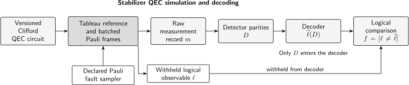
A QEC simulation pipeline. The stabilizer engine executes a versioned Clifford circuit and sampled Pauli faults, then exposes measurement-derived detectors and a declared logical observable. The decoder receives only its allowed detector data, returns a predicted frame, and is scored by the corrected logical outcome.

Pauli Noise and Its Boundary

A stochastic Pauli channel has the form

$$\mathcal N(\rho) = \sum_{P\in\mathcal P_n} p_P P\rho P, \qquad p_P\geq0, \qquad \sum_P p_P=1.$$

One trajectory samples $P$ and adds it to the frame. Independent single-location faults, correlated multi-qubit Pauli faults, measurement flips, reset faults, and erasure flags can all be represented if their joint event probabilities and timing are explicit.

Not every physical noise process is a Pauli channel. Pauli twirling a coherent rotation produces a different channel that may match selected average quantities while removing coherent accumulation. Leakage leaves the qubit Pauli space. Amplitude damping is not a mixture of Pauli conjugations. Slow drift and non-Markovian correlations require a context model beyond independent fault draws.

Stabilizer simulation may still contribute to a hybrid treatment, but the model change must be named. Noise in Quantum Information owns the physical taxonomy and error metrics. A dedicated noise-simulation page owns general channel, density-matrix, and trajectory strategies.

Pauli Noise and Depolarizing Channels owns the declared Pauli-law, transfer-eigenvalue, Clifford-propagation, syndrome/logical-pushforward, and twirling-adequacy contract; this page retains simulator representations, sampling algorithms, detector streams, performance engineering, and run validation.

From Measurements to Detectors

Repeated QEC circuits produce many raw ancilla measurements. A detector is a declared parity that is deterministic in the reference circuit. Let $m_k$ be measurement bits. Detector $a$ is

$$d_a = b_a \oplus \bigoplus_{k\in S_a} m_k,$$

where $S_a$ identifies the included measurements and $b_a$ sets the expected reference parity. A detection event occurs when $d_a=1$.

For repeated measurement of one stabilizer check, an interior detector often compares consecutive rounds,

$$d_{r,j} = m_{r,j}\oplus m_{r-1,j}.$$

Boundary detectors may also include preparation or final data measurements. Their definitions depend on the experiment. A simulator should not infer them from names or geometry when an explicit parity specification is available.

Detector coordinates, times, and logical associations are metadata for a decoder. They do not change the quantum state, but mistakes in that metadata change the inferred logical performance. Noiseless simulation should verify that all declared deterministic detectors are zero for every allowed reference branch.

Decoder Interface and Logical Failure

The simulator and decoder are different components.

• The simulator samples a circuit under a declared model and emits detector data plus logical-observable data reserved for scoring.
• The decoder receives only its allowed detector data and model metadata.
• The decoder predicts a correction class or logical frame.
• The evaluator compares that prediction with the withheld logical outcome.

Let $\ell\in\{0,1\}^k$ be the simulated logical-observable flips and $\widehat\ell(D)$ the decoder’s prediction from detector record $D$. A logical failure indicator is

$$f = \mathbf 1 \left[ \ell\oplus\widehat\ell(D) \neq \mathbf 0 \right].$$

Giving the decoder the sampled physical error or the true logical flip leaks ground truth and invalidates the experiment. Decoder weights may use the declared noise model, but training, tuning, and final evaluation data should be separated.

The interface should version:

• detector ordering, coordinates, and boundary conventions;
• logical-observable definitions and basis;
• circuit rounds, resets, and final-measurement mapping;
• decoder graph or model and edge probabilities;
• erasure or side-information fields;
• postselection and discarded-shot rules;
• output correction convention and tie breaking.

Estimating Logical Error Rates

For $N$ independent shots with $K$ failures,

$$\widehat p_L = \frac{K}{N}.$$

The uncertainty is binomial only when shots are independent and identically distributed under the declared fixed model. Shared drift, reused random contexts, adaptive stopping, or correlated batches change the statistical analysis.

When $K=0$, reporting $p_L=0$ is wrong. A one-sided upper confidence limit at confidence $1-\delta$ is

$$p_L \leq 1-\delta^{1/N}.$$

At 95 percent confidence this is approximately $3/N$ for large $N$, the so-called rule of three. Resolving very small logical error rates therefore requires enormous shot counts or a validated rare-event method such as importance sampling or splitting.

Threshold studies should report physical-noise parameters, circuit and decoder, code distances, shot allocation, confidence intervals, finite-size fitting, and stopping rules. A crossing of two finite-distance curves is evidence within that protocol and noise model, not a universal hardware threshold.

Quantum Error Correction and Fault Tolerance freezes the code, fault, extraction, decoder, estimand, and evidence records before an executable experiment; this page retains the tableau engine, Pauli frames, detector generation, decoder interface, batched sampling, performance engineering, and numerical validation.

QEC Simulation Workflow

1. Freeze the experiment contract

Specify code geometry, number of rounds, syndrome circuit, operation schedule, initial logical state, final logical measurement, detectors, observables, noise model, decoder, and success rule. Hash the executable circuit and detector model.

2. Run noiseless semantic checks

All reference detectors should have their declared deterministic values. The logical observable should match the prepared state. Exercise every boundary and every classically controlled branch. This catches sign, order, and final- readout mistakes before statistical sampling.

3. Inject single faults exhaustively

For small and moderate circuits, place each supported elementary fault at each location. Record its detector pattern and logical effect. This verifies fault timing, propagation, detector definitions, and distance claims. Distinct faults may share a detector pattern because decoding is an inference problem.

4. Sample multi-fault shots

Draw faults from the frozen joint model, propagate frames, and produce detector records. Keep simulator runtime, output serialization, and decoder runtime separate. Preserve enough seed and batch metadata to reproduce any failed shot.

5. Decode without privileged information

Pass only allowed features to the decoder. Apply the predicted logical frame under one declared convention. Count failures and stratify them by context, distance, basis, and fault count when useful.

6. Validate and report uncertainty

Compare a subset against an independent tableau or state-vector backend. Compute confidence intervals. Repeat across seed families and check that results are stable under batch size and parallel scheduling. For approximate decoders or rare-event sampling, validate the additional approximation separately.

Performance Engineering

Separate analysis from sampling

Many workloads have a one-time circuit-analysis phase and a repeated-shot phase. Analysis may build an inverse tableau, detector-error model, fault-to- detector map, or reference sample. Sampling then propagates frames or sparse events. Report both times and the break-even shot count; quoting only steady- state samples per second hides startup cost.

Pack across qubits or shots

Tableau simulation often packs Pauli coordinates across words. Bulk error sampling can instead pack the same fault or measurement bit across many shots, so one machine-word XOR updates dozens or hundreds of trajectories. These layouts optimize different axes and may require a transpose between analysis and sampling.

Exploit sparse faults carefully

Below threshold, most locations do not fault. Event-based sampling can draw only the nontrivial mechanisms and propagate their effects. Correlated events, mutually exclusive mechanisms, and heralded erasures must preserve their joint probabilities. Replacing a correlated mechanism with independent sparse faults changes the model.

Output can dominate

A simulator producing billions of detector bits can become limited by memory allocation, compression, or I/O rather than Clifford algebra. Streaming shots directly to a decoder avoids materializing the full sample matrix. If data are compressed or detectors are reordered, the schema and permutation belong in the result record.

Benchmark the actual workload

Report qubits, gates, measurements, resets, rounds, detectors, logical observables, fault mechanisms, shots, representation, word width, threads, hardware, analysis time, sampling time, decoder time, peak memory, and output policy. A gate-only random Clifford benchmark does not characterize a measurement-heavy surface-code experiment.

Near-Clifford Extensions

Non-Clifford resources break basic tableau closure, but a small amount of nonstabilizer structure can sometimes be handled by decomposition. Write

$$\lvert\psi\rangle = \sum_{a=1}^{\chi} c_a\lvert\phi_a\rangle,$$

where each $\lvert\phi_a\rangle$ is a stabilizer state. Clifford gates update each term efficiently; runtime and memory grow with the stabilizer rank $\chi$, overlap calculations, and branching. For many magic resources, $\chi$ can grow exponentially.

Quasiprobability methods decompose nonstabilizer channels into signed or complex-weighted stabilizer operations and estimate observables by weighted sampling. They can be unbiased while suffering variance that grows with the decomposition overhead. “Uses stabilizer simulation” does not therefore imply polynomial total sample complexity.

Near-Clifford algorithms are valuable for circuits with limited magic and for benchmarking non-Clifford gadgets. Their error and cost contracts should state whether the decomposition is exact or approximate, how coefficients are chosen, what quantity is estimated, and how variance or truncation is bounded.

One non-Clifford gate does not make every finite instance hard. It removes the general closure guarantee and introduces a resource whose scaling must be analyzed.

Verification and Validation

Structural invariants

• Stabilizer rows must commute and remain independent when a pure state is claimed.
• Stabilizer and destabilizer rows must preserve their declared symplectic pairing.
• Clifford updates must preserve the symplectic form and valid phase domain.
• Reset and measurement must leave a valid postmeasurement tableau.

Analytic fixtures

• Prepare computational, Bell, GHZ, and graph states and query their known Pauli expectations.
• Measure known stabilizers for deterministic outcomes and anticommuting Paulis for balanced outcomes.
• Apply a random Clifford and its inverse.
• Propagate isolated Pauli frames through $H$, $S$, CNOT, and measurement.
• Check both bit and eigenvalue output conventions.

Differential checks

Compare small stabilizer circuits with the exact state-vector method from Quantum Circuit Simulation. Use an independent gate table, parser path, and random-number implementation where possible. Compare final states up to global phase, measurement probabilities, conditional branches, and detector records.

QEC-specific fixtures

• Every noiseless detector has its declared reference value.
• Exhaustive single faults produce reviewed detector and logical patterns.
• Equivalent Pauli representatives produce the same logical class.
• Decoder inputs exclude hidden faults and withheld logical labels.
• A decoder-correction convention is tested on known correctable errors.
• Parallel and serial sampling agree statistically under the same seed policy.

Reproducible Run Record

A mature run should preserve:

• circuit and detector-model hashes and schema versions;
• qubit, measurement, detector, and logical-observable ordering;
• Pauli coordinate, phase, and measurement-bit conventions;
• simulator implementation, representation, version, and compilation options;
• circuit-analysis artifacts and whether their cost was amortized;
• exact fault mechanisms, probabilities, correlations, and timing;
• random generator, root seed, stream derivation, batches, and shot count;
• decoder implementation, graph or model hash, weights, and tie-breaking rule;
• postselection, erasure handling, and discarded-shot counts;
• failures, confidence intervals, stopping rules, and rare-event weights;
• hardware, threads, memory, analysis time, sample time, decoder time, and I/O;
• independent validation results and known model limitations.

The record should distinguish ideal stabilizer simulation, stochastic Pauli noise simulation, and approximation of a non-Pauli physical process. Those three support different scientific claims.

Common Mistakes

• Repeating the full state-vector simulation of a large Clifford circuit and overlooking polynomial stabilizer structure.
• Treating phase bits as disposable because global phase is unobservable.
• Calling destabilizer rows additional physical stabilizers.
• Assuming every Pauli measurement is random or every syndrome measurement is deterministic.
• Mixing measurement bits with eigenvalues without the mapping $\lambda=(-1)^m$.
• Applying every Pauli correction instead of tracking a frame when later operations permit frame propagation.
• Describing a Pauli-twirled coherent error as the original physical channel.
• Modeling leakage, damping, or drift as Pauli faults without stating and validating the approximation.
• Giving a decoder the sampled physical error or withheld logical label.
• Reporting zero logical error after observing zero failures.
• Quoting samples per second while excluding circuit analysis or decoder time.
• Treating a finite-distance curve crossing as a universal threshold.
• Exporting raw measurements without versioned detector and boundary parities.
• Assuming efficient sampling implies efficient enumeration of every output probability or amplitude.
• Claiming one non-Clifford gate automatically makes a specific instance hard.

Exercises

1. Compare representation sizes

Estimate the raw storage of a $2n\times(2n+1)$ binary tableau at $n=1{,}000$. Compare it conceptually with a double-complex state vector.

Solution

The tableau contains

$$2{,}000\times2{,}001 = 4{,}002{,}000$$

bits, or $500{,}250$ bytes, approximately $0.477$ MiB before alignment, scratch space, and object overhead. The state vector would contain $2^{1000}$ complex amplitudes and is physically impossible to store. The comparison does not imply that every 1,000-qubit stabilizer workload is fast; circuit and sample counts still matter.

2. Classify a Bell measurement

The Bell state $\lvert\Phi^+\rangle$ is stabilized by $X_1X_2$ and $Z_1Z_2$. Is a measurement of $Z_1$ deterministic or random? What correlations remain?

Solution

$Z_1$ anticommutes with $X_1X_2$, so the measurement is random with equal probability for bits $m=0$ and $m=1$. After the measurement, the state is $\lvert00\rangle$ for $m=0$ and $\lvert11\rangle$ for $m=1$. Equivalently, the postmeasurement stabilizers can be chosen as $(-1)^m Z_1$ and $Z_1Z_2$, which imply the same eigenvalue for $Z_2$.

3. Propagate a Pauli frame

An $X$ frame error is present on the control before a CNOT from $Q_1$ to $Q_2$. The circuit then applies $H$ to $Q_2$. What is the final frame?

Solution

Under CNOT conjugation,

$$X_1 \longmapsto X_1X_2.$$

The later Hadamard maps $X_2$ to $Z_2$, so the final frame is

$$X_1Z_2.$$

No physical correction had to be inserted; the simulator updates the binary frame and flips later measurement bits when this frame anticommutes with the measured observable.

4. Construct repeated-round detectors

A noiseless check has measurement bit $1$ in every round because the prepared state is in its $-1$ eigenspace. Should the interior detector be $d_r=m_r\oplus m_{r-1}$ or simply $d_r=m_r$?

Solution

Use the parity $d_r=m_r\oplus m_{r-1}$. It is zero when the repeated result is stable, regardless of whether the reference eigenvalue is $+1$ or $-1$. Defining $d_r=m_r$ would report a detection event in every noiseless round. Boundary detectors still need explicit offsets or preparation/final data terms.

5. Score a decoder

For two logical observables, a shot has true logical-flip vector $\ell=(1,0)$ and the decoder predicts $\widehat\ell=(1,1)$. Does the shot fail under the any-logical-error rule?

Solution

The residual is

$$\ell\oplus\widehat\ell = (0,1),$$

which is nonzero. Therefore $f=1$ and the shot is a logical failure. A study may also report per-observable rates, but the aggregate rule must be declared before evaluation.

6. Bound a zero-failure result

A simulation observes no logical failures in $N=10^6$ independent shots. Give the approximate one-sided 95 percent upper bound rather than reporting zero.

Solution

Using the rule of three,

$$p_L \lesssim \frac{3}{10^6} = 3\times10^{-6}.$$

The exact binomial expression is $1-0.05^{1/10^6}$, which is very close to this value. The claim depends on independent identically distributed shots and the frozen model.

7. Diagnose a twirling claim

A coherent overrotation is replaced by a Pauli channel with a matched average infidelity, and the stabilizer simulation reports a logical error rate. What must the conclusion say?

Solution

It is the logical error rate of the Pauli-twirled model, not automatically of the original coherent overrotation. Matching average infidelity does not preserve coherent accumulation, temporal correlations, or every logical observable. The approximation should be validated against a coherent-noise method on accessible sizes or bounded analytically for the intended circuit.

8. Find decoder leakage

A decoder input table contains detector bits, detector coordinates, and the exact sampled Pauli fault at every circuit location. Why is the resulting logical-error estimate invalid?

Solution

The exact sampled faults are privileged ground truth unavailable to a real decoder. They can reveal the correction directly, bypassing the inference from syndrome data. Fault labels may be retained for auditing and failure analysis, but the decoder-facing schema must exclude them unless the physical experiment would genuinely provide equivalent side information.

9. Estimate near-Clifford growth

Suppose each of $t$ non-Clifford gadgets doubles the number of stabilizer terms in a naive exact decomposition. How many terms are present, and what does this show?

Solution

The naive expansion contains

$$\chi=2^t$$

stabilizer terms. Each term evolves efficiently through later Clifford gates, but the number of terms is exponential in the non-Clifford count. Stabilizer simulation remains a useful inner kernel; it does not by itself make the full near-Clifford algorithm polynomial in $t$.

Research Status

Tableau and graph-state simulation of ideal stabilizer circuits is mature. Modern implementations substantially improve practical performance through inverse tableaus, SIMD bit packing, reference samples, batched Pauli frames, sparse fault mechanisms, and streaming detector interfaces. Exact performance still depends on circuit structure, measurement density, representation, and requested output.

Stabilizer simulation is central to large-scale QEC design because syndrome circuits, Pauli faults, frame tracking, and many decoding experiments fit its closed subtheory. Active work includes faster circuit-to-detector analysis, more expressive correlated-fault models, rare-event estimation, decoder- simulator co-design without information leakage, dynamic logical circuits, erasure and leakage hybrids, and reproducible threshold workflows.

Near-Clifford simulation remains active. Stabilizer decompositions, quasiprobability sampling, tensor-network hybrids, and magic monotones seek to extend the tractable region. Their utility is instance and output dependent; variance, stabilizer rank, or contraction width replaces tableau size as the dominant resource.

Further Connections

• Stabilizer Formalism is the canonical home for Pauli symplectic algebra, stabilizer codes, tableau semantics, measurement updates, and the Gottesman–Knill theorem.
• Quantum Circuit Simulation supplies the general simulation task, exact state-vector baseline, measurement semantics, resource accounting, and validation ladder.
• Randomized Benchmarking uses Clifford-group sampling and compiled inverses; stabilizer tools can validate ideal sequence construction and efficiently generate reference fixtures without replacing a noise model.
• Shadow Tomography uses efficiently represented random Clifford states for global shadows and contrasts them with shallow local-Pauli acquisition.
• Tensor-Network Simulation exploits contraction width and bounded bond dimension rather than Clifford closure and supports circuit families and near-Clifford hybrids outside the tableau contract.
• Noise Simulation places high-throughput Pauli-fault execution within the wider choice among density, trajectory, tensor, leakage, and memory-bearing noise engines.
• Why Quantum Error Correction Is Possible explains syndrome extraction, correctable error sets, recovery, logical channels, and the assumptions behind protection.
• Surface Code develops the code geometry, repeated checks, boundaries, logical strings, decoding problem, and threshold interpretation used in major stabilizer workloads.
• Universal Gate Sets separates Clifford closure from the non-Clifford resources needed for universal quantum computation.
• Noise in Quantum Information distinguishes Pauli, coherent, leakage, correlated, and non-Markovian noise and the metrics used to compare them.
• Stabilizer Circuit is the compact model card for the efficiently simulable operation set.
• Stabilizer Identities collects the main formulas and conventions for quick reference.

References

1. D. Gottesman, “Stabilizer codes and quantum error correction,” PhD thesis, California Institute of Technology (1997), arXiv:quant-ph/9705052.
2. D. Gottesman, “The Heisenberg representation of quantum computers,” in Group22: Proceedings of the XXII International Colloquium on Group Theoretical Methods in Physics, 32–43 (1999), arXiv:quant-ph/9807006.
3. S. Aaronson and D. Gottesman, “Improved simulation of stabilizer circuits,” Physical Review A 70, 052328 (2004), doi:10.1103/PhysRevA.70.052328.
4. S. Anders and H. J. Briegel, “Fast simulation of stabilizer circuits using a graph-state representation,” Physical Review A 73, 022334 (2006), doi:10.1103/PhysRevA.73.022334.
5. C. Gidney, “Stim: a fast stabilizer circuit simulator,” Quantum 5, 497 (2021), doi:10.22331/q-2021-07-06-497.
6. S. Bravyi and D. Gosset, “Improved classical simulation of quantum circuits dominated by Clifford gates,” Physical Review Letters 116, 250501 (2016), doi:10.1103/PhysRevLett.116.250501.
7. S. Bravyi, D. Browne, P. Calpin, E. Campbell, D. Gosset, and M. Howard, “Simulation of quantum circuits by low-rank stabilizer decompositions,” Quantum 3, 181 (2019), doi:10.22331/q-2019-09-02-181.
8. H. Pashayan, J. J. Wallman, and S. D. Bartlett, “Estimating outcome probabilities of quantum circuits using quasiprobabilities,” Physical Review Letters 115, 070501 (2015), doi:10.1103/PhysRevLett.115.070501.
9. E. Dennis, A. Kitaev, A. Landahl, and J. Preskill, “Topological quantum memory,” Journal of Mathematical Physics 43, 4452–4505 (2002), doi:10.1063/1.1499754.
10. O. Higgott, “PyMatching: a Python package for decoding quantum codes with minimum-weight perfect matching,” ACM Transactions on Quantum Computing 3, article 16 (2022), doi:10.1145/3505637.
11. O. Higgott and C. Gidney, “Sparse Blossom: correcting a million errors per core second with minimum-weight matching,” Quantum 9, 1600 (2025), doi:10.22331/q-2025-01-20-1600.
12. M. A. Nielsen and I. L. Chuang, Quantum Computation and Quantum Information, 10th anniversary ed., Cambridge University Press (2010), doi:10.1017/CBO9780511976667.