Noise Simulation

Short Definition

Noise simulation is the numerical execution of a quantum circuit or continuous-time process under a declared nonideal model. The model may contain quantum channels, Lindblad generators, stochastic Pauli faults, coherent offsets, leakage states, classical drift, correlated events, or an explicit environment with memory.

The result is a prediction of the model, not of the physical device without qualification:

$$\text{simulation output} = \text{model prediction} + \text{numerical and statistical error}.$$

Agreement with hardware is a separate validation question. A simulation can be numerically exact and physically misleading because the model omits crosstalk, leakage, drift, or temporal correlations. It can also use a well-calibrated model but be numerically unreliable because of coarse time steps, density-matrix positivity loss, tensor truncation, or insufficient trajectories.

This page owns method selection, binding noise to a compiled circuit timeline, density-operator and trajectory execution, structure-aware backends, correlated-noise orchestration, uncertainty accounting, performance, and cross-method validation. Noise in Quantum Information owns the device-facing taxonomy. Common Noise Models owns model cards and parameter conventions.

Dephasing and Amplitude Damping owns the qualified T1–T2 and thermal-population conversion, one-step physicality, composition, and adequacy contract; this page retains numerical representations, event scheduling, sampling algorithms, correlated-noise orchestration, performance engineering, and run validation.

Leakage and Crosstalk owns the physical-space, survival-branch, leakage/seepage/coherence, flag, scalar-license, operational-context, and composition contract; this page retains numerical representations, multilevel and correlated propagation, event scheduling, sampling algorithms, performance engineering, uncertainty, and run validation.

The Quantum Channels and Noise volume owns Kraus, Choi, dilation, and complete-positivity theory. The open-systems trajectory and notebook pages own individual derivations and small reproducible examples.

Freeze the Simulation Contract

Noise, Channels, and Error Mitigation freezes the mechanism, representation, context, estimand, evidence, intervention, and resource question before computation; this page retains executable channel and trajectory propagation, uncertainty sampling, numerical verification, and reproducibility.

Quantum Channels for QI owns representation selection, conversion, physicality checks, and composition conventions; this page retains algorithms, matrix-free execution, trajectories, uncertainty sampling, performance, and numerical cross-validation.

A noisy-circuit job should identify:

• the compiled circuit, qubit map, schedule, gate parameters, and timing;
• the simulated Hilbert space, including leakage or loss sectors;
• preparations, resets, measurements, and classical feedforward;
• every noise mechanism, parameter convention, placement, and correlation;
• model version, calibration snapshot, and validity interval;
• requested outputs and whether they are exact values or samples;
• execution method, precision, tolerances, and random-seed policy;
• comparison target, uncertainty budget, and acceptance test.

Noise attaches to implemented events, not abstract source gates. Routing adds operations and idles. Simultaneous gates alter context. Pulse duration sets exposure to relaxation and dephasing. A model bound before compilation can therefore describe a different timeline from the one executed.

Let $\mathcal U_k$ denote the ideal channel of operation $k$. One possible Markovian placement convention is

$$\rho_{k+1} = \mathcal E^{\mathrm{post}}_{k,c_k} \circ \mathcal U_k \circ \mathcal E^{\mathrm{pre}}_{k,c_k} (\rho_k),$$

where context $c_k$ may include duration, neighbors, concurrent operations, and calibration epoch. A different order generally gives a different result. “One percent noise per gate” is incomplete until the channel and placement are specified.

Preparations, Instruments, and Readout

State-preparation and measurement errors should not be hidden inside every gate channel. A terminal measurement with ideal outcomes $x$ and a classical readout response $R(y\mid x)$ gives

$$p(y) = \sum_x R(y\mid x) \operatorname{Tr} \left( M_x\rho_{\mathrm{out}} \right).$$

Here $M_x$ is the quantum POVM element and $R$ is a classical conditional probability matrix. This factorization is useful only if detector backaction, leakage-dependent readout, crosstalk, and history dependence are negligible or modeled elsewhere.

Mid-circuit measurements require quantum instruments, not only outcome confusion. An instrument branch $\mathcal I_m$ determines both

$$p(m) = \operatorname{Tr} \left[ \mathcal I_m(\rho) \right]$$

and the conditioned state

$$\rho_m = \frac{ \mathcal I_m(\rho) }{ p(m) }.$$

Classical feedforward then selects later operations using the simulated reported bit, which may differ from an underlying detector state. Reset must say whether it is an ideal replacement, measurement plus feedback, dissipative preparation, or a fitted channel.

SPAM Errors owns the QI-facing actual-preparation, effect/instrument, assignment-license, identifiability, gauge, context-transfer, and validated-mitigation contract; this page retains numerical state/channel/instrument representations, event scheduling, correlated sampling, performance engineering, uncertainty, and run validation.

Exact Density-Operator Propagation

For Hilbert-space dimension $d$, a density operator has $d^2$ complex entries. For $n$ qubits,

$$d = 2^n, \qquad d^2 = 4^n.$$

Dense density propagation is the most direct general method for small Markovian circuits. It represents mixtures exactly for the declared channels, returns expectation values without trajectory sampling error, and provides a reference backend for other methods.

For Kraus operators satisfying

$$\sum_\alpha K_\alpha^\dagger K_\alpha = I,$$

the channel update is

$$\rho' = \mathcal E(\rho) = \sum_\alpha K_\alpha\rho K_\alpha^\dagger.$$

Apply local operators directly to tensorized density data when possible. Constructing a full superoperator often costs much more memory than applying its terms.

Liouville-space form

Under column-stacking vectorization,

$$\operatorname{vec} \left( A\rho B \right) = \left( B^{\mathsf T} \otimes A \right) \operatorname{vec}(\rho).$$

Therefore

$$\operatorname{vec} \left[ \mathcal E(\rho) \right] = \mathsf S_{\mathcal E} \operatorname{vec}(\rho), \qquad \mathsf S_{\mathcal E} = \sum_\alpha K_\alpha^* \otimes K_\alpha.$$

This form turns channel composition into matrix multiplication and time-independent master equations into linear ordinary differential equations. But $\mathsf S_{\mathcal E}$ is a $d^2\times d^2$ matrix with $d^4$ entries. Matrix-free action is essential except at small $d$.

Vectorization order is part of the interface. Row stacking changes the Kronecker formula. A silent convention mismatch can preserve dimensions while producing incorrect dynamics.

Numerical invariants

At checkpoints, test

$$\operatorname{Tr}\rho = 1, \qquad \rho = \rho^\dagger, \qquad \lambda_{\min}(\rho) \geq 0$$

within declared tolerances. Tiny negative eigenvalues can arise from roundoff; large or systematic negativity indicates a bad map, integrator, truncation, or implementation. Clipping eigenvalues and renormalizing changes the state and must not be used as silent repair.

Stochastic Kraus Trajectories

A channel acting on a pure state can be sampled one Kraus branch at a time. For state $\lvert\psi\rangle$,

$$p_\alpha = \langle\psi\rvert K_\alpha^\dagger K_\alpha \lvert\psi\rangle,$$

and branch $\alpha$ updates the normalized state to

$$\lvert\psi_\alpha\rangle = \frac{ K_\alpha\lvert\psi\rangle }{ \sqrt{p_\alpha} }.$$

The ensemble recovers the channel:

$$\sum_\alpha p_\alpha \lvert\psi_\alpha\rangle \langle\psi_\alpha\rvert = \mathcal E \left( \lvert\psi\rangle\langle\psi\rvert \right).$$

A full circuit trajectory samples branches at successive noisy locations while retaining only a state vector. Its memory scales as $O(2^n)$ instead of $O(4^n)$, but many independent trajectories may be needed.

For an observable outcome $X_r$ from trajectory $r$,

$$\widehat\mu = \frac1N \sum_{r=1}^{N} X_r, \qquad \widehat{\operatorname{SE}} (\widehat\mu) = \frac{s_X}{\sqrt N},$$

where $s_X$ is the sample standard deviation. Parallelism reduces wall time, not statistical uncertainty at fixed $N$.

Kraus representations and variance

A channel has many Kraus representations. They produce the same ensemble density operator when sampled correctly, but individual trajectories and estimator variance can differ. If trajectories are only a numerical device, the representation may be chosen for efficiency and variance reduction. If they are interpreted as physical monitored records, the corresponding unraveling and environment measurement must be specified.

Unravelings owns this physical distinction. Quantum Jump Simulation and Diffusive Trajectory Simulation own the small-system algorithms and convergence demonstrations.

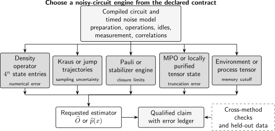
A noise-simulation contract. A versioned compiled timeline and declared model are routed to an engine suited to the model structure and requested output. Every route must expose model limitations, numerical or truncation error, sampling uncertainty, and independent validation before producing a qualified claim.

Continuous-Time Lindblad Simulation

For a Markovian time-local model, the density operator obeys the Lindblad–GKSL equation. Lindblad–GKSL Equation owns its derivation and validity assumptions. Numerically, one can:

• integrate the density-matrix equation directly;
• apply an exponential or exponential-action of the Liouvillian;
• split coherent and dissipative generators;
• sample quantum-jump or diffusive trajectories;
• use structured tensor or sparse representations.

For jump operators $L_j$ and rates $\gamma_j$, the effective no-jump Hamiltonian is

$$H_{\mathrm{eff}} = H - \frac{i\hbar}{2} \sum_j \gamma_j L_j^\dagger L_j.$$

Over a small interval $\Delta t$, jump $j$ has probability

$$p_j = \gamma_j\Delta t \langle L_j^\dagger L_j \rangle + O(\Delta t^2).$$

A discrete jump algorithm must control the probability of multiple jumps within one step or use waiting-time sampling. A density ODE solver must control time discretization and stiffness. Generic high-order ODE accuracy does not automatically preserve complete positivity at every finite step.

When gates have finite duration, the Hamiltonian and dissipator may act simultaneously. Applying an ideal unitary and then a gate-independent channel is a splitting approximation unless it is the declared phenomenological model. Validate convergence in $\Delta t$ and compare splitting orders.

Solving Lindblad Equations owns vectorized Liouvillians, ODE versus exponential comparisons, stationary states, and small analytic solver fixtures.

Pauli and Stabilizer Noise

A stochastic Pauli channel samples a Pauli fault with its declared probability. If preparations, gates, measurements, feedforward, and faults all remain in the stabilizer contract, a tableau or Pauli-frame simulator can execute very large noisy circuits efficiently.

Stabilizer Simulation owns batched Pauli frames, detector streams, decoder isolation, and logical error experiments. The method is exact for the stated stochastic Pauli model. It is not exact for an untwirled coherent rotation, amplitude damping, general leakage, or arbitrary non-Clifford gates.

Pauli twirling can produce a useful comparison model, but it removes coherent phase relations. Matching average gate infidelity does not guarantee matching logical error, long-sequence behavior, or worst-case error. Report results as predictions of the twirled model.

Structured Mixed-State Methods

Dense $4^n$ storage is often prohibitive before a pure state vector is. Structure-aware alternatives include:

• matrix-product operators and matrix-product density operators;
• locally purified tensor networks;
• stochastic pure-state MPS trajectories;
• tensor contraction of channel or doubled circuit networks;
• sparse Liouvillians and symmetry blocks;
• low-rank density factorizations.

An MPO compresses a density operator according to operator-space entanglement, not ordinary pure-state entanglement alone. Truncating an MPO can break positivity even when trace and Hermiticity look acceptable. Locally purified forms encode

$$\rho = X X^\dagger$$

and preserve positivity by construction, but both spatial and purification bond dimensions can grow.

Tensor-Network Simulation owns circuit tensorization, contraction trees, slicing, and MPS error contracts. A noisy extension must additionally report:

• operator or purification bond dimensions;
• positivity-preserving parameterization;
• channel and environment truncations;
• trace and normalization policy;
• convergence of the requested noisy observable or distribution.

Noise can suppress long-range coherence and make some instances easier, but this is not universal. Weak noise may leave large operator entanglement, and a small output error at one noise strength does not establish favorable asymptotic scaling.

Leakage, Loss, and Enlarged State Spaces

A qubit-only channel cannot represent population in $\lvert2\rangle$ unless leakage is replaced by an effective qubit model. To simulate leakage directly, enlarge the local Hilbert space and define:

• computational and leakage projectors;
• leakage and seepage transitions;
• gates acting on every retained level;
• measurement response for leaked states;
• reset behavior and any heralding;
• truncation of higher levels and its convergence.

For $n$ local systems of dimension $q$, dense state and density sizes become

$$q^n \quad\text{and}\quad q^{2n},$$

respectively. Raising a transmon model from two to three levels therefore changes memory exponentially with $n$. Hybrid treatments may track a classical leakage flag with conditional qubit dynamics, but the approximation and allowed return paths must be explicit.

Loss and erasure are not synonymous. Erasure supplies a trusted location flag; unheralded loss does not. Postselecting lost shots changes the simulated experiment and requires acceptance probability as an output.

Correlated Noise and Memory

A product of independent per-location channels assumes that the future noise depends only on declared present context. It cannot represent arbitrary history dependence.

Classical latent processes

Slow drift or correlated control offsets can be represented by a latent classical process $\theta_t$. Sample a complete context path and condition operations on it:

$$\rho_{k+1} = \mathcal E_{k,\theta_k} \circ \mathcal U_k(\rho_k).$$

Drawing an independent $\theta_k$ at every gate destroys the intended temporal correlation. Conversely, drawing one offset for an entire run models quasistatic noise, not rapidly fluctuating noise. The covariance or transition law is part of the model.

Explicit environments

A channel can be dilated as

$$\mathcal E(\rho) = \operatorname{Tr}_E \left[ V \left( \rho\otimes \lvert0\rangle\langle0\rvert_E \right) V^\dagger \right].$$

Refreshing the environment after each step yields a memoryless construction. Retaining and reusing environment degrees of freedom can generate memory, but their Hilbert space and entanglement may grow rapidly. An environment reset is a physical modeling choice, not a free numerical cleanup.

Process tensors and influence functionals

A multitime process tensor maps a sequence of interventions to later outcomes. It can represent temporal correlations that no fixed sequence of independent channels captures. Tensor-network influence-functional methods compress memory along the time direction when temporal correlations decay sufficiently.

The resources are memory time, time discretization, and temporal bond dimension. Cutting memory or truncating the influence MPO is an approximation that needs convergence tests. What Non-Markovian Means owns the conceptual distinctions among memory, divisibility, information backflow, and microscopic approximations.

Markovian and Non-Markovian Noise owns the empirical license for fixed-step, interval-specific, hidden-state, enlarged-system, or process-tensor models; this page retains numerical representations, event scheduling, correlated sampling, solver engineering, uncertainty, and run validation.

Parameter Uncertainty and Nested Sampling

Calibrated noise parameters are estimates, not exact constants. Let $\theta$ denote uncertain model parameters and $\omega$ the simulator’s trajectory randomness. A predictive mean has the nested form

$$\mu = \mathbb E_{\theta} \left[ \mathbb E_{\omega\mid\theta} \left[ X(\theta,\omega) \right] \right].$$

Using only a point estimate $\widehat\theta$ omits calibration uncertainty and can understate tails. A practical study may sample parameter draws from a posterior, bootstrap, or confidence region, then run trajectories within each draw.

Separate:

• variation across model parameters;
• Monte Carlo error within a fixed parameter draw;
• hardware shot noise in the validation data;
• drift between calibration and experiment.

Common random numbers can reduce variance when comparing two circuits or model parameters, but paired estimates are correlated. Confidence intervals must use the paired design rather than pretending every result is independent.

Error and Uncertainty Ledger

At least six layers can contribute:

Layer	Example	Control
model discrepancy	omitted crosstalk or memory	held-out hardware validation and richer models
parameter uncertainty	uncertain $T_1$, rates, or readout matrix	calibration ensembles and sensitivity analysis
time discretization	coarse Lindblad or stochastic step	step refinement and higher-quality integrators
representation approximation	MPO, purification, or environment truncation	bond and memory convergence
trajectory sampling	finite stochastic ensemble	standard errors and independent seed families
floating-point error	cancellation or positivity drift	precision checks and stable kernels

These errors do not generally add as independent variances. Report each component under its own assumptions. If a rigorous bound is unavailable, give a convergence or sensitivity study rather than an invented combined error bar.

Model discrepancy is often dominant and is not reduced by running more trajectories.

Method Selection

Workload	Good first method	Limiting resource
small general Markovian circuit	dense density matrix	$4^n$ storage and local channel cost
moderate circuit, many stochastic channels	pure-state trajectories	$2^n$ state and estimator variance
Clifford circuit with Pauli faults	stabilizer or Pauli-frame sampling	departures from Clifford and Pauli closure
one-dimensional structured open circuit	MPDO, purification, or MPS trajectories	operator, purification, or state bond dimension
time-local driven open system	density ODE or quantum jumps	stiffness, step error, and trajectory count
leakage-aware few-qudit system	enlarged dense density matrix	local dimension raised to system size
quasistatic or classically correlated noise	latent-context trajectories	context sampling and correlation model
non-Markovian bath with finite memory	explicit environment or process-tensor method	environment size, memory time, temporal bond
final readout confusion only	ideal quantum evolution plus classical response	validity of the factorization

The requested output can change the choice. A density matrix is attractive for many observables at small width. Independent trajectories are attractive for a few estimators and parallel hardware. Full output probabilities remain exponentially large even when each trajectory is manageable.

Performance and Reproducibility

Record:

• compiled circuit and schedule hashes;
• physical-to-logical qubit map and local dimensions;
• noise-model schema, version, parameters, uncertainty, and validity window;
• channel placement, composition order, timing, and correlation scope;
• simulator method, representation, precision, tolerance, and backend version;
• trajectories, shots, root seed, stream derivation, batching, and stopping rule;
• density, state, operator, purification, environment, and temporal bond dimensions as applicable;
• time steps, integrator, splitting order, and solver tolerances;
• path-search or tensor-contraction metadata where applicable;
• wall time, peak memory, devices, communication, and output policy;
• invariant checks, cross-method comparisons, convergence data, and held-out hardware validation.

For trajectories, make results invariant in distribution under thread count and batching. Counter-based or hierarchically derived streams can make each trajectory reproducible without forcing one serial execution order. Replaying one seed is useful for debugging; statistical conclusions require independent seed families.

Verification and Validation

Local model checks

• Verify Kraus completeness, Choi positivity, and parameter domains.
• Check the identity limit as every error parameter tends to zero.
• Verify fixed points, unitality, and conserved quantities where expected.
• Compare channel composition with analytic one-qubit results.
• Confirm leakage, loss, and readout conventions on basis states.

Solver checks

• Compare density, superoperator, and trajectory methods on small circuits.
• Compare quantum-jump ensembles with direct Lindblad evolution.
• Compare Pauli trajectories with stabilizer execution on Clifford fixtures.
• Refine time steps, trajectory counts, tensor bonds, and memory cutoffs.
• Run alternate precisions and reduction orders.
• Track trace, Hermiticity, positivity, normalization, and symmetry leakage.

End-to-end checks

• Validate compiled timing and noise placement against the executable schedule.
• Hold out circuits, depths, contexts, and calibration epochs from model fitting.
• Compare more than one summary metric: populations, coherences, correlators, leakage, and output distributions when feasible.
• Test deliberate falsifiers such as simultaneous gates, long idles, repeated cycles, and echo sequences.
• Report where the model fails, not only where it was tuned.

A model that reproduces its calibration circuits has passed an internal consistency check, not an independent predictive test.

Common Mistakes

• Calling a noisy simulation a simulation of the device without naming the fitted model and validation domain.
• Attaching noise to source gates before routing, scheduling, and duration are known.
• Omitting whether a channel acts before, after, or during a gate.
• Using a full $d^4$ superoperator when matrix-free Kraus action is sufficient.
• Assuming a density-matrix result has no uncertainty because it has no trajectory sampling.
• Reporting trajectory means without standard errors or independent seeds.
• Treating one Kraus trajectory as a physical history without specifying an unraveling.
• Sampling a fresh drift parameter at every gate when the model is quasistatic.
• Twirling coherent noise and reporting the result as the untwirled model.
• Representing leakage in a qubit-only Hilbert space without naming the effective approximation.
• Clipping negative density eigenvalues silently.
• Treating generic ODE accuracy as a guarantee of complete positivity.
• Omitting acceptance probability when loss or postselection discards shots.
• Ignoring parameter uncertainty because the calibration returned point estimates.
• Using the same circuits to fit and validate a model.
• Claiming that more trajectories reduce model discrepancy.

Exercises

1. Price a dense density matrix

How much raw memory does a complex128 density matrix require for $n=15$ qubits, before scratch space and alignment?

Solution

The matrix contains

$$4^{15} = 2^{30} = 1{,}073{,}741{,}824$$

complex entries. At 16 bytes per complex128 value, this is

$$2^{30}\times16 = 2^{34}\ \mathrm{bytes} = 16\ \mathrm{GiB}.$$

A practical update may need the input, output, Kraus workspaces, and temporary permutations simultaneously, so 16 GiB is not a sufficient machine-memory budget.

2. Sample amplitude damping

For amplitude damping with

$$K_0 = \begin{pmatrix} 1&0\\ 0&\sqrt{1-\gamma} \end{pmatrix}, \qquad K_1 = \begin{pmatrix} 0&\sqrt\gamma\\ 0&0 \end{pmatrix},$$

find the trajectory probabilities for $\lvert\psi\rangle=a\lvert0\rangle+b\lvert1\rangle$.

Solution

The jump probability is

$$p_1 = \langle\psi\rvert K_1^\dagger K_1 \lvert\psi\rangle = \gamma |b|^2.$$

The no-jump probability is

$$p_0 = |a|^2 + (1-\gamma)|b|^2 = 1-\gamma|b|^2.$$

On a jump, the normalized state is $\lvert0\rangle$. On no jump, it is

$$\frac{ a\lvert0\rangle + \sqrt{1-\gamma}\,b\lvert1\rangle }{ \sqrt{p_0} }.$$

Averaging the two branch projectors gives the usual amplitude-damping channel.

3. Show that placement matters

Start in $\lvert0\rangle$. Compare an ideal $X$ gate followed by amplitude damping of strength $\gamma$ with amplitude damping followed by $X$.

Solution

Applying $X$ first prepares $\lvert1\rangle$. Damping then gives

$$\rho_A = \gamma \lvert0\rangle\langle0\rvert + (1-\gamma) \lvert1\rangle\langle1\rvert.$$

Damping $\lvert0\rangle$ does nothing, and the later $X$ gives

$$\rho_B = \lvert1\rangle\langle1\rvert.$$

Thus $\rho_A\neq\rho_B$ for $\gamma>0$. A channel name and probability do not define a circuit model without composition order.

4. Estimate trajectory uncertainty

A binary logical-failure estimator observes $K=240$ failures in $N=20{,}000$ independent trajectories. Estimate the rate and its standard error using the binomial plug-in variance.

Solution

The estimate is

$$\widehat p = \frac{240}{20{,}000} = 0.012.$$

The estimated standard error is

$$\widehat{\operatorname{SE}} = \sqrt{ \frac{ \widehat p(1-\widehat p) }{ N } } \approx 7.7\times10^{-4}.$$

A report should use an appropriate binomial interval rather than treating $\widehat p\pm2\,\widehat{\operatorname{SE}}$ as exact in every regime.

5. Apply a readout response

An ideal measurement gives $p(x=1)=0.3$. The readout flips $0\to1$ with probability $0.02$ and $1\to0$ with probability $0.08$. Find the reported probability $p(y=1)$.

Solution

Using the classical response,

$$p(y=1) = 0.02\,p(x=0) + 0.92\,p(x=1).$$

Since $p(x=0)=0.7$,

$$p(y=1) = 0.02(0.7) + 0.92(0.3) = 0.29.$$

This postprocessing is valid only under the declared factorization between quantum evolution and classical readout confusion.

6. Preserve quasistatic correlation

Every gate in one circuit run has the same random overrotation $\delta\sim\mathcal N(0,\sigma^2)$. Why is drawing a fresh $\delta_k$ for every gate a different model?

Solution

The quasistatic model has

$$\operatorname{Cov} (\delta_j,\delta_k) = \sigma^2$$

for every pair of gates in the run. Independent draws have zero covariance for $j\neq k$. The first model allows coherent accumulation of one persistent offset; the second tends to randomize accumulation. To simulate quasistatic noise, draw one $\delta$ per run or per declared correlation block.

7. Diagnose a density-matrix repair

A solver returns a trace-one Hermitian matrix with minimum eigenvalue $-3\times10^{-3}$, then clips negative eigenvalues and renormalizes. Why is this not a satisfactory validation procedure?

Solution

The negativity is far larger than ordinary complex128 roundoff for a well-conditioned small calculation. It may indicate a non-CP map, excessive time step, bad vectorization, or truncation error. Clipping changes the state, can bias observables, and hides the source. The solver should refine its step, check the local channels and conventions, compare with a positivity-preserving method, and report any explicit projection as an approximation.

8. Separate two error sources

Doubling the number of trajectories changes an estimate little, but halving the Lindblad time step shifts it substantially. Which error currently dominates, and what convergence study is needed?

Solution

The observed sensitivity points to time-discretization or splitting error, not trajectory variance. Continue refining $\Delta t$ under at least two solver or splitting orders and check the output against a direct density solution on a tractable instance. Only after the deterministic result is stable is increasing trajectory count the relevant route to smaller Monte Carlo uncertainty.

9. Audit a hardware-matching claim

A noisy simulator matches device output on the same circuits used to fit its depolarizing probabilities. What additional evidence is needed before calling the model predictive?

Solution

Use held-out circuits that vary depth, idles, gate concurrency, routing, initial states, measurement bases, and calibration epoch. Compare populations, coherences or correlators, leakage, and distributions where feasible, with hardware shot uncertainty included. Challenge the independent depolarizing assumption using echo, simultaneous-gate, repeated-cycle, and drift-sensitive fixtures. Training-set agreement alone establishes fit consistency.

Research Status

Dense channel propagation, Lindblad solvers, Monte Carlo wave functions, and standard stochastic trajectories are mature. Their mathematical equivalence under stated Markovian assumptions is well established, and production software supports sparse, parallel, and time-dependent variants.

The practical frontier lies in scale and model fidelity. Active directions include variance-reduced unravelings, distributed trajectory execution, positivity-preserving tensor networks, operator-space compression, correlated fault sampling, differentiable noisy simulators, uncertainty propagation, hardware-aware model learning, and process-tensor methods for finite-memory dynamics.

No one backend is a universal reference. Dense density matrices lose to exponential memory; trajectories lose to estimator variance; stabilizer methods lose generality; tensor methods lose to growing bond dimensions; finite-memory methods lose to long correlations. Trustworthy results identify the favorable structure, show convergence within it, and test the model outside its fitting set.

Further Connections

• Quantum Circuit Simulation supplies the ideal baseline, output-task taxonomy, dynamic-circuit semantics, and cross-method validation ladder.
• Noise in Quantum Information develops coherent, incoherent, leakage, crosstalk, SPAM, drift, and correlation mechanisms.
• Common Noise Models provides model cards, parameter conversions, placement warnings, and falsification tests.
• Simulating Quantum Channels specifies small Kraus, Choi, composition, and complete-positivity notebook fixtures.
• Solving Lindblad Equations specifies density ODE, Liouvillian, steady-state, and finite-time-channel checks.
• Quantum Jump Simulation and Diffusive Trajectory Simulation provide focused stochastic notebook contracts.
• Stabilizer Simulation owns high-throughput Clifford and Pauli-fault execution for QEC.
• Tensor-Network Simulation owns MPS and spacetime contraction machinery reused by structured noisy methods.

References

1. G. Lindblad, “On the generators of quantum dynamical semigroups,” Communications in Mathematical Physics 48, 119–130 (1976), doi:10.1007/BF01608499.
2. V. Gorini, A. Kossakowski, and E. C. G. Sudarshan, “Completely positive dynamical semigroups of N-level systems,” Journal of Mathematical Physics 17, 821–825 (1976), doi:10.1063/1.522979.
3. J. Dalibard, Y. Castin, and K. Mølmer, “Wave-function approach to dissipative processes in quantum optics,” Physical Review Letters 68, 580–583 (1992), doi:10.1103/PhysRevLett.68.580.
4. R. Dum, P. Zoller, and H. Ritsch, “Monte Carlo simulation of the atomic master equation for spontaneous emission,” Physical Review A 45, 4879–4887 (1992), doi:10.1103/PhysRevA.45.4879.
5. M. B. Plenio and P. L. Knight, “The quantum-jump approach to dissipative dynamics in quantum optics,” Reviews of Modern Physics 70, 101–144 (1998), doi:10.1103/RevModPhys.70.101.
6. H.-P. Breuer and F. Petruccione, The Theory of Open Quantum Systems, Oxford University Press (2002), doi:10.1093/acprof:oso/9780199213900.001.0001.
7. J. R. Johansson, P. D. Nation, and F. Nori, “QuTiP 2: A Python framework for the dynamics of open quantum systems,” Computer Physics Communications 184, 1234–1240 (2013), doi:10.1016/j.cpc.2012.11.019.
8. A. H. Werner et al., “Positive tensor network approach for simulating open quantum many-body systems,” Physical Review Letters 116, 237201 (2016), doi:10.1103/PhysRevLett.116.237201.
9. F. A. Pollock et al., “Non-Markovian quantum processes: Complete framework and efficient characterization,” Physical Review A 97, 012127 (2018), doi:10.1103/PhysRevA.97.012127.
10. M. R. Jørgensen and F. A. Pollock, “Exploiting the causal tensor network structure of quantum processes to efficiently simulate non-Markovian path integrals,” Physical Review Letters 123, 240602 (2019), doi:10.1103/PhysRevLett.123.240602.
11. C. Gidney, “Stim: a fast stabilizer circuit simulator,” Quantum 5, 497 (2021), doi:10.22331/q-2021-07-06-497.
12. S. Cheng et al., “Simulating noisy quantum circuits with matrix product density operators,” Physical Review Research 3, 023005 (2021), doi:10.1103/PhysRevResearch.3.023005.
13. S. V. Isakov et al., “Simulations of quantum circuits with approximate noise using qsim and Cirq” (2021), arXiv:2111.02396.
14. M. A. Nielsen and I. L. Chuang, Quantum Computation and Quantum Information, 10th anniversary ed., Cambridge University Press (2010), doi:10.1017/CBO9780511976667.