Tensor-Network Simulation

Short Definition

Tensor-network circuit simulation rewrites a quantum circuit and its requested output as a network of indexed tensors, then evaluates that network without materializing every amplitude of the quantum state. It is useful when the circuit has a favorable spatial ordering, limited entanglement, low depth, small separators, reusable substructure, or a contraction path whose largest intermediate tensor fits available resources.

The method does not make arbitrary large circuits easy. Exact cost can still grow exponentially with contraction width, while approximate state methods can require exponentially growing bond dimension. The defensible claim is:

A specified output of a specified circuit was evaluated under a measured contraction-width, bond-dimension, memory, and error contract.

Qubit count alone is not that contract.

This page owns circuit-to-network translation, matrix-product-state execution, spacetime contraction, contraction-path search, index slicing, output-aware sampling, dynamic-circuit branches, simulator performance, and validation. Tensor Networks Preview owns the graph-and-index language, virtual gauges, cut-capacity bounds, and the MPS–PEPS–MERA family map. Tensor Networks: Computational Guide owns convergence design for many-body state calculations. Quantum Circuit Simulation owns the general simulator contract and exact state-vector baseline.

From a Circuit to a Tensor Network

Consider an ideal $n$-qubit circuit

$$U_C = U_L U_{L-1}\cdots U_1$$

acting on $\lvert 0^n\rangle$. A selected output amplitude is

$$A_C(x) = \langle x\rvert U_C \lvert 0^n\rangle.$$

Write every preparation, gate, and final bra as an array with one index for each incident wire segment. Joining two wire segments means summing their shared basis label. The amplitude is then the complete contraction of this network.

For example, a two-qubit gate contributes components

$$G^{a'b'}_{ab} = \langle a'b'\rvert G \lvert ab\rangle.$$

The lower indices meet tensors before the gate and the upper indices meet tensors after it. Fixing an output bit attaches either $\langle0\rvert$ or $\langle1\rvert$. Leaving an output index open asks for a vector of amplitudes rather than one scalar.

The conversion is exact. Difficulty enters when deciding:

• which output legs remain open;
• which pairs or groups of tensors contract first;
• which indices are sliced into independent subproblems;
• whether an intermediate state or environment is compressed;
• what numerical precision and reduction order are used.

Those choices belong to the executable simulation artifact, not merely to an implementation note.

Gate tensors are not all dense

A generic two-qubit unitary is a rank-four tensor with local dimension two. But identity, diagonal, permutation, controlled, matchgate, Clifford, and symmetry-blocked tensors contain additional structure. A simulator may exploit that structure through sparse kernels, block labels, symbolic simplification, or specialized factorizations.

The optimization must preserve semantics. Replacing a gate by a low-rank approximation changes the circuit unless an approximation and error bound are declared. Merely reshaping or exactly factorizing a gate does not.

The Requested Output Defines the Network

There is no single tensor network associated with a circuit independent of the question being asked.

Task	Boundary tensors	Result
selected amplitude	fix every output bit	$A_C(x)$
batch of amplitudes	leave selected output legs open	tensor indexed by those bits
selected probability	contract one amplitude and take its squared magnitude	$p_C(x)$
marginal probability	join a ket and bra network and sum unobserved outputs	$p_C(x_S)$
expectation value	insert $O$ between ket and bra networks	$\langle O\rangle$
reduced density operator	leave ket and bra legs of a subsystem open	$\rho_S$
weak sample	evaluate a sequence of conditional probabilities	$x\sim p_C$

For a subset $S$ of measured qubits,

$$p_C(x_S) = \sum_{x_{\bar S}} \left| A_C(x_S,x_{\bar S}) \right|^2.$$

This is naturally a doubled network containing $U_C$, $U_C^\dagger$, output projectors on $S$, and identity contractions on $\bar S$. Many gate pairs outside the causal cone cancel exactly in such doubled networks. Contracting a full state first and discarding most of it may waste the very structure the method is intended to use.

Output size is also a lower bound. Leaving $k$ binary legs open produces $2^k$ complex numbers. A clever path cannot store or transmit an explicitly requested dense object in subexponential space.

Two Main Execution Views

Tensor-network circuit simulators commonly organize the same algebra in two different ways.

State boundary moving through time

The simulator represents the current state as an MPS or another tensor-network state and applies gates in circuit order. The boundary between contracted and uncontracted circuit layers moves forward in time. Compression keeps the state representation within a selected bond dimension.

This view is attractive when:

• qubits admit a good one-dimensional ordering;
• gates are local or can be applied without excessive swaps;
• entanglement across that ordering remains controlled;
• many final observables or samples will reuse the evolved state;
• dynamic measurements are handled one trajectory at a time.

Spacetime contraction

The simulator constructs the whole network for the requested scalar or tensor and chooses an arbitrary contraction tree. The order need not follow circuit time. It may contract within light cones, across space, through time, or in a hybrid pattern.

This view is attractive when:

• only a few amplitudes, probabilities, or observables are required;
• the circuit is shallow on a wide graph;
• a small separator exists in the spacetime network;
• slicing exposes many independent tasks;
• intermediate contractions can be reused across output batches.

Neither view dominates universally. An MPS sweep is itself a particular contraction strategy with controlled intermediate factorization. A spacetime path may locally create MPS-like boundaries. The practical distinction is what is materialized, when compression occurs, and which reuse pattern is favored.

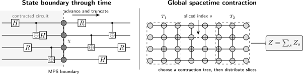
Two execution views of the same circuit algebra. A state-evolution method moves an MPS boundary through gate layers and may truncate its bond dimension $\chi$. A spacetime method chooses a global contraction tree and may slice an internal index $s$ to fit memory and distribute independent subproblems.

Matrix-Product-State Circuit Execution

For local dimension $q$, an open-boundary MPS has amplitudes

$$\Psi_{s_1\cdots s_n} = \sum_{\alpha_1,\ldots,\alpha_{n-1}} A^{[1]s_1}_{\alpha_1} A^{[2]s_2}_{\alpha_1\alpha_2} \cdots A^{[n]s_n}_{\alpha_{n-1}}.$$

The bond at cut $j$ has dimension $\chi_j$. In an exact canonical MPS, $\chi_j$ is the Schmidt rank across $\{1,\ldots,j\}\mid\{j+1,\ldots,n\}$. A uniform upper bound $\chi_j\leq\chi$ gives storage of order

$$M_{\mathrm{MPS}} = O(nq\chi^2)$$

for dense tensors, compared with $O(q^n)$ amplitudes in a state vector.

Applying a two-qubit gate

For adjacent sites $j$ and $j+1$, contract their tensors with the gate to form a temporary object

$$\Theta^{s'_j s'_{j+1}}_{\alpha\beta} = \sum_{s_j,s_{j+1},\gamma} G^{s'_j s'_{j+1}}_{s_j s_{j+1}} A^{[j]s_j}_{\alpha\gamma} A^{[j+1]s_{j+1}}_{\gamma\beta}.$$

Reshape $\Theta$ into a matrix with row index $(\alpha,s'_j)$ and column index $(s'_{j+1},\beta)$, compute an SVD, and redistribute the factors into the two site tensors. Keeping every nonzero singular value makes the update exact up to floating-point roundoff. Keeping at most $\chi_{\max}$ values makes it approximate.

For uniform $q$ and $\chi$, a dense two-site update commonly costs on the order of $q^3\chi^3$, with constants depending on gauges, gate factorization, and matrix shapes. This polynomial statement is useful only while $\chi$ remains controlled.

Entanglement is the operative resource

If a gate crossing a cut has operator Schmidt rank $r_G$, then

$$\chi'_j \leq r_G\chi_j, \qquad r_G\leq q^2.$$

For qubits, a generic crossing gate can therefore multiply the exact Schmidt rank by as much as four. Repeated layers can drive $\chi$ exponentially with depth even though every gate is local.

Conversely, many nominally wide circuits remain tractable because their actual Schmidt spectra decay rapidly, gates rarely cross the chosen ordering, or symmetries split the tensors into smaller blocks. Entanglement entropy gives the necessary bound

$$S_j \leq \log \chi_j,$$

but entropy alone does not determine truncation accuracy. The full tail of the Schmidt spectrum matters.

Truncation and its local meaning

Let the normalized post-gate Schmidt coefficients be $s_1\geq s_2\geq\cdots$. If values beyond $\chi_{\max}$ are removed, the discarded weight is

$$\epsilon_{\mathrm{disc}} = \sum_{a>\chi_{\max}} s_a^2.$$

For that one truncation, the normalized retained state has fidelity

$$F_{\mathrm{local}} = 1-\epsilon_{\mathrm{disc}}$$

with the untruncated post-gate state. This clean local statement does not make the sum of discarded weights an exact global infidelity after many nonlinear truncate-and-renormalize steps. Cumulative discarded weight is a diagnostic. Global claims require bond-dimension convergence, exact checks on accessible instances, or a separate error analysis.

Ordering and nonlocal gates

An MPS chooses a one-dimensional ordering even when hardware connectivity is two-dimensional or irregular. A gate between distant MPS sites can be applied by:

• inserting and later undoing SWAPs;
• moving an orthogonality center and using a nonlocal update;
• dynamically changing the site ordering;
• factorizing the gate into an MPO;
• switching to another network geometry or a spacetime contraction.

All can be exact before truncation, but their intermediate bond dimensions and data movement differ. The hardware layout is therefore not automatically the best MPS ordering. A simulator should record the ordering and every dynamic reordering.

Spacetime Contraction and Contraction Trees

Suppose tensors $A$ and $B$ carry index sets $I$ and $J$, with shared indices $K=I\cap J$. Their pairwise contraction is

$$C_{(I\cup J)\setminus K} = \sum_K A_I B_J.$$

For dense indices of dimensions $d_e$, a rough multiply-add count is

$$W(A,B) \sim \prod_{e\in I\cup J} d_e,$$

while the output tensor contains

$$\left|C\right| = \prod_{e\in (I\cup J)\setminus K} d_e$$

elements. A contraction tree recursively chooses which intermediate tensors to combine until the requested output remains.

The total work is the sum over tree nodes, whereas peak memory depends on simultaneously live inputs, outputs, workspaces, and parallel tasks. Minimizing the largest intermediate alone need not minimize wall time. A path with slightly more FLOPs can run faster if it produces balanced matrix multiplications and less index permutation.

Width and treewidth

For binary indices, an operational memory-width measure is

$$w_{\mathrm{mem}} = \log_2 \left( \max_T |T| \right),$$

where the maximum runs over intermediate tensors in a chosen path. Exact runtime is exponentially sensitive to related separator widths. Graph treewidth and the treewidth of an associated line graph formalize this connection for common contraction models.

Markov and Shi showed that circuits of size $T$ and suitable graph treewidth $d$ can be simulated in time

$$T^{O(1)} \exp[O(d)].$$

This is a structural result, not a promise that a heuristic will find the best path cheaply or that every low-depth circuit has small width under every connectivity graph.

Path search is part of the algorithm

Finding an optimal contraction sequence is computationally hard. Practical optimizers combine:

• greedy local scoring;
• graph or hypergraph partitioning;
• tree decompositions;
• stochastic search and simulated annealing;
• subtree reconfiguration;
• Bayesian or other hyperparameter optimization;
• hardware-aware penalties for memory, communication, and kernel shape.

Path-search time can be negligible for one small network or substantial for a large repeated workload. Report it separately and state whether the path is reused across circuit instances, output bitstrings, parameters, or shots.

Exact simplification before path search

Useful exact preprocessing includes:

• absorbing rank-one preparation and projection tensors;
• fusing chains of one-qubit gates;
• canceling $U^\dagger U$ pairs outside an observable’s causal cone;
• removing dimension-one indices and scalar factors;
• recognizing diagonal, copy, permutation, and sparse tensors;
• exposing symmetry sectors and conserved charges;
• decomposing high-rank gates when the factorization is exact.

Simplification changes the graph seen by the path optimizer and can matter as much as the optimizer itself. Every rewrite should be unit tested against the unsimplified network on small instances.

Index Slicing and Distributed Execution

If a path exceeds memory, choose internal indices $S$ and fix their values. The original contraction becomes

$$Z = \sum_{s\in\Omega_S} Z_s, \qquad |\Omega_S| = \prod_{e\in S}d_e.$$

Each $Z_s$ is a smaller network with the sliced indices removed. Complete summation is algebraically exact and the slices can be evaluated independently. This makes slicing a natural route to clusters and accelerators.

The tradeoff is not free:

• more slices reduce per-task memory;
• duplicated contractions can increase total work;
• load can vary among slices when dimensions or sparsity differ;
• partial tensors may be reusable across related slices;
• the final reduction can lose precision through cancellation;
• task count and output traffic can overwhelm a scheduler.

A good plan chooses contraction order and slicing jointly. Report the sliced indices, number of slices, estimated and measured work overhead, concurrency, per-worker peak memory, reduction precision, and whether deterministic summation is required.

For complex values with $b$ bytes per element, a first memory estimate is

$$M_{\mathrm{peak}} \gtrsim b \max_T |T|,$$

but production planning must include simultaneously live tensors, temporary permutations, library workspaces, cached environments, and concurrent slices. An element-count estimate is not a measured resident-set size.

Amplitudes, Marginals, and Sampling

One amplitude versus many

Fixing all output legs often yields a compact scalar network. Computing $10^6$ unrelated amplitudes by repeating that contraction can be wasteful. Options include:

• leave $k$ output legs open and obtain $2^k$ amplitudes per contraction;
• cache a prefix or subtree shared by many bitstrings;
• partition bitstrings into batches with common fixed outputs;
• form an approximate final state with a declared fidelity;
• use a direct conditional-sampling scheme.

The best choice depends on output count, memory, contraction width, and whether amplitudes are needed as values or only as a route to samples.

Sequential sampling from an MPS

A normalized canonical MPS supports exact direct sampling, up to roundoff and any prior truncation. Draw bits from

$$p(s_j\mid s_1,\ldots,s_{j-1}) = \frac{ p(s_1,\ldots,s_j) }{ p(s_1,\ldots,s_{j-1}) }.$$

After drawing $s_j$, contract the selected physical slice into the running environment and continue. No Markov-chain equilibration is needed. Reusing the final MPS makes many samples much cheaper than rebuilding the circuit.

The implementation should clip only tiny negative probabilities attributable to a documented roundoff tolerance, renormalize conditionals carefully, and fail loudly when normalization defects exceed that tolerance.

Sampling from a general contraction

A general spacetime network can also sample sequentially by contracting marginals or conditional networks. Naively, this requires many expensive contractions per bit and per shot. Cached environments, multi-output contractions, prefix trees, and specialized sampling constructions can reuse work.

“One amplitude is tractable” does not imply that a million independent samples are tractable. Conversely, an algorithm designed to generate many samples may not expose every exact amplitude. The simulator capability must name the actual output primitive.

Mid-Circuit Measurement and Feedforward

A measurement branch inserts a projector $P_m$ and has probability

$$p(m) = \langle\psi\rvert P_m \lvert\psi\rangle.$$

For one trajectory, sample $m$, condition the state or network on that value, renormalize, and execute the classically selected successor operations. An MPS trajectory updates its state boundary. A spacetime method can fix the measured leg and rebuild or specialize the remaining network.

Enumerating every branch may grow exponentially in the number of random measurements. Trajectory sampling avoids constructing the entire branch tree, but obtaining each conditional probability can still be expensive. Prefix reuse helps when many shots share early outcomes.

The circuit contract must define:

• measurement bit versus eigenvalue conventions;
• whether outcomes are terminal, retained, or discarded;
• reset semantics;
• allowed classical expressions and timing;
• postselection and zero-probability branches;
• random-seed hierarchy and parallel reproducibility.

General noisy channels, density-operator networks, purification growth, and trajectory unravelings belong to the planned noise-simulation article. A pure state truncated to small bond dimension is not a noise model unless a specific, validated approximation says so.

Exactness and Approximation Ledger

Several choices that are often conflated have different scientific meanings.

Choice	Exact in algebra?	Main consequence
contraction order	yes	time, memory, communication, roundoff order
complete index slicing	yes	more parallel tasks and often more total work
exact tensor factorization	yes	changed graph and kernel shapes
MPS bond truncation	no	state approximation
approximate boundary environment	no	contraction approximation
omitting slices	generally no	biased or incomplete contraction unless justified
reduced precision	no in real arithmetic	numerical roundoff and possible instability
causal-cone cancellation	yes when preconditions hold	smaller network

For an approximate output, select a metric that matches the claim:

• state infidelity $1-|\langle\psi\vert\phi\rangle|^2$;
• norm error $\lVert\psi-\phi\rVert$;
• absolute amplitude error $|A-\widetilde A|$;
• observable error $|\langle O\rangle-\widetilde{\langle O\rangle}|$;
• total-variation distance

$$D_{\mathrm{TV}}(p,\widetilde p) = \frac12 \sum_x \left| p(x)-\widetilde p(x) \right|.$$

Relative amplitude error is ill conditioned near an exact or accidental zero. A small energy error need not control a sampling distribution. A high cross-entropy score need not establish small total-variation distance. Match the validation quantity to the intended use.

Method Selection

Workload	Good first candidate	Audit first
local one-dimensional circuit with moderate entanglement	MPS gate evolution	maximum and converged bond dimensions
shallow circuit on a wide sparse graph	spacetime contraction	path width, path-search cost, slicing
a few selected amplitudes	fixed-output spacetime network	reuse and cancellation
many samples from one retained low-entanglement state	canonical MPS sampling	truncation and conditional normalization
local observable in a larger circuit	doubled causal-cone contraction	exact cancellation and environment error
large Clifford circuit	stabilizer simulator	whether all operations stay in the stabilizer contract
deep volume-law circuit	state vector, hybrid, or carefully costed tensor method	evidence that tensor structure survives
dynamic circuit	trajectory MPS or branch-aware contraction	conditional-cost and branch reuse

Method selection should occur after the output is fixed. The same circuit may favor MPS for repeated samples, a spacetime contraction for one amplitude, and a state vector for all amplitudes at moderate width.

Performance and Reproducibility Contract

A tensor-network benchmark should record:

• canonical circuit IR, hash, parameter values, qubit ordering, and gate semantics;
• requested outputs, open and fixed legs, measurement branch, and precision;
• exact simplifications and gate factorizations;
• network graph, index dimensions, symmetry blocks, and tensor sparsity;
• MPS site order, gauges, maximum bond dimensions, truncation rule, and discarded-weight history;
• contraction optimizer, objective, random seed, trials, search time, and final tree;
• estimated FLOPs, largest intermediate, sliced indices, task count, and reuse plan;
• hardware, accelerator type, threads, processes, library versions, and communication topology;
• measured wall time by path search, preprocessing, contraction, reduction, sampling, and output;
• peak resident memory per worker and aggregate temporary storage;
• numerical precision, accumulation precision, normalization policy, and deterministic-reduction setting;
• validation fixtures, exact comparison sizes, convergence data, and known failure regimes.

“FLOPs” and “seconds” are not interchangeable. Tensor contractions with the same operation count can have very different arithmetic intensity, transpose traffic, communication, and accelerator utilization. Both modeled resources and measured execution belong in a credible report.

Verification and Validation

Semantic fixtures

• Compare one- and two-qubit gates against reviewed matrices under the same index order.
• Contract Bell, GHZ, and product-state circuits with known amplitudes, marginals, and correlators.
• Check $U^\dagger U$ circuits and classically controlled inverse branches.
• Verify open-leg ordering by comparing a small emitted amplitude tensor with the state-vector basis order.

Cross-method checks

• Compare small circuits with the exact state-vector backend.
• Compare Clifford-only instances with Stabilizer Simulation.
• Evaluate the same network with several contraction trees.
• Sum all slices and compare with an unsliced contraction where memory permits.
• Compare MPS and spacetime methods on overlapping tractable workloads.

Exact contraction trees should agree within a precision-dependent tolerance. Disagreement beyond roundoff indicates an index, conjugation, reduction, or implementation error, not a legitimate “method difference.”

Approximation checks

• increase $\chi_{\max}$ and record output-level convergence;
• vary truncation thresholds independently of hard bond caps;
• compare multiple qubit orderings;
• vary boundary-environment dimensions and contraction approximations;
• test observables with different support and amplitudes near cancellation;
• measure normalization and symmetry leakage;
• compare samples by marginals, moments, and distributional tests on sizes where exact probabilities are available.

Convergence at two nearby bond dimensions is weak evidence when both lie below an entanglement-growth transition. Use multiple values, independent methods, and deliberately hard fixtures.

Common Mistakes

• Describing tensor networks as polynomial merely because each input gate is a small tensor.
• Reporting qubit count without depth, connectivity, output task, contraction width, or bond dimension.
• Treating a heuristic contraction path as an approximation to the numerical answer; a complete path changes cost, not algebra.
• Treating omitted slices as exact slicing.
• Calling cumulative discarded weight the exact final-state infidelity.
• Assuming low entropy guarantees a rapidly decaying Schmidt spectrum at the required tolerance.
• Ignoring the qubit ordering used by an MPS.
• Applying many SWAPs for nonlocal gates without charging their entanglement and runtime cost.
• Recontracting every requested amplitude or sample without considering cached environments or open output legs.
• Building a full doubled network when causal-cone cancellation removes most of it.
• Comparing FLOP estimates with measured device time as though they were the same metric.
• Excluding path-search, slicing overhead, tensor transposes, or output I/O from a performance claim.
• Using relative error for amplitudes close to zero.
• Describing a truncated pure-state calculation as physical decoherence.
• Claiming quantum advantage from the failure of one tensor-network ordering, optimizer, bond cap, or hardware implementation.

Exercises

1. Contract a Bell amplitude

The circuit prepares $\lvert00\rangle$, applies $H$ to qubit 1, and then CNOT with qubit 1 as control. Express the amplitude for output $x_1x_2$ as an index contraction and evaluate it.

Solution

Let $a$ be the basis index between $H$ and CNOT. Then

$$A(x_1x_2) = \sum_{a=0}^{1} \langle x_1x_2\rvert \mathrm{CNOT} \lvert a0\rangle \langle a\rvert H\lvert0\rangle.$$

CNOT maps $\lvert a0\rangle$ to $\lvert aa\rangle$, so the first factor is $\delta_{x_1,a}\delta_{x_2,a}$. Since both $\langle0\rvert H\lvert0\rangle$ and $\langle1\rvert H\lvert0\rangle$ equal $1/\sqrt2$,

$$A(00) = A(11) = \frac{1}{\sqrt2}, \qquad A(01) = A(10) = 0.$$

The joined index $a$ is precisely the contracted wire segment.

2. Estimate a pairwise contraction

Tensor $A_{ijk}$ has dimensions $(2,4,8)$ and tensor $B_{k\ell m}$ has dimensions $(8,3,5)$. Estimate the output size and dense multiply-add count for contracting over $k$.

Solution

The output $C_{ij\ell m}$ has

$$2\times4\times3\times5 = 120$$

elements. Each output sums over eight values of $k$, so the rough dense work is

$$2\times4\times8\times3\times5 = 960$$

multiply-add pairs. This local estimate does not include index permutation, allocation, or the effect on later intermediates.

3. Bound Schmidt-rank growth

An MPS has Schmidt rank $\chi=64$ across a cut. A two-qubit gate crossing that cut has operator Schmidt rank $r_G=2$. What upper bound follows for the exact post-gate rank? Does the rank have to reach the bound?

Solution

The operator-Schmidt expansion writes the gate as a sum of two product operators across the cut. Acting on a state of Schmidt rank 64 therefore gives rank at most

$$\chi' \leq r_G\chi = 128.$$

The actual rank may be smaller because terms can be linearly dependent or have zero weight for the particular state. The bound controls worst-case growth; it does not predict the Schmidt spectrum.

4. Interpret discarded weight

A normalized two-site update has squared Schmidt coefficients $0.70$, $0.20$, $0.08$, and $0.02$. If only two values are kept, find the discarded weight and the one-step fidelity after renormalization.

Solution

The discarded weight is

$$\epsilon_{\mathrm{disc}} = 0.08+0.02 = 0.10.$$

The normalized retained state has one-step fidelity

$$F_{\mathrm{local}} = 1-\epsilon_{\mathrm{disc}} = 0.90.$$

This does not say that ten such truncations produce final fidelity $(0.90)^{10}$ or $1-10(0.10)$. Later gates and truncations act on changed states, so a global claim needs a separate analysis.

5. Price a slicing plan

A contraction exceeds memory. You slice five binary indices. How many subproblems result, and what must be true for their sum to equal the unsliced answer?

Solution

Five binary indices produce

$$N_{\mathrm{slice}} = 2^5 = 32$$

subproblems. Every assignment must be evaluated under the same original network semantics and all 32 results must be summed. Omitting assignments, changing tensor normalization between slices, or using an uncontrolled reduction changes the result. Slicing can reduce peak memory while increasing total work through duplicated contractions.

6. Choose an output strategy

You need $2^{12}$ amplitudes that share all output bits except a selected 12-qubit subset. Why might leaving those output legs open be better than running $2^{12}$ independent scalar contractions?

Solution

One contraction with 12 open binary legs can reuse every intermediate that is independent of those outputs and return a tensor with $2^{12}$ entries. Scalar repetition may redo that shared work. The open-leg plan is not automatically better: its intermediates may be larger, and the $2^{12}$-entry output must still be stored. Compare complete contraction trees and measured resource costs for both plans.

7. Sample a GHZ MPS

For

$$\lvert\mathrm{GHZ}_n\rangle = \frac{ \lvert0^n\rangle + \lvert1^n\rangle }{ \sqrt2 },$$

what are the left-to-right conditional probabilities?

Solution

The first bit is uniform:

$$p(s_1=0) = p(s_1=1) = \frac12.$$

After drawing $s_1$, every later bit is deterministic:

$$p(s_j=s_1\mid s_1,\ldots,s_{j-1}) = 1$$

for $j>1$. Direct MPS sampling therefore returns only $0^n$ and $1^n$, each with probability one half, without a Markov chain.

8. Classify exact and approximate choices

A simulator uses a heuristic contraction path, slices three indices and sums every slice, performs all contractions in complex128, and never truncates a tensor. Which parts are approximations?

Solution

The heuristic path and complete slicing are algebraically exact. “Heuristic” means the cost may not be optimal, not that the contraction omits terms. Complex128 introduces floating-point roundoff, so the computed result is not exact over the real numbers. There is no bond or environment approximation in the stated procedure. Validation should compare alternate paths or a reference calculation at a tolerance consistent with conditioning and precision.

9. Audit a simulation claim

A report states: “We exactly simulated a 500-qubit circuit using tensor networks.” Name at least six additional facts needed to assess the claim.

Solution

At minimum ask for circuit depth and topology; gate set and parameters; requested output; input and measurement conditions; contraction or MPS strategy; largest intermediate or bond dimension; whether any truncation, slice omission, or low-fidelity model was used; numerical precision; total path-search and execution time; peak memory and hardware; and independent validation. A 500-qubit product circuit may be trivial, while a much smaller deep circuit can be prohibitive.

Research Status

The exact mapping from circuits to tensor networks and the relation between contraction complexity and graph width are established. MPS simulation of limited-entanglement circuits is mature, as are exact contraction, slicing, and direct sampling from contractible network states.

The practical frontier remains active. Contraction-tree search, hypergraph partitioning, hardware-aware cost models, distributed slicing, intermediate reuse, mixed precision, symmetry handling, and direct multi-sample algorithms continue to improve. Modern classical reassessments of quantum-processor experiments repeatedly show why simulation baselines must be updated and why claims must specify the output task and accuracy.

Approximate tensor-network simulation of deep two-dimensional circuits is especially instance dependent. Success may come from a favorable Schmidt spectrum, treelike correlations, a narrow causal cone, a low-fidelity target, or an observable much easier than the full state. Failure of one ansatz or path is not evidence that all classical methods fail, and success on one observable does not imply faithful recovery of the full output distribution.

Further Connections

• Quantum Circuit Simulation defines output tasks, state-vector kernels, measurement semantics, broad method selection, and the simulator evidence contract.
• Tensor Networks Preview owns tensors, graphs, virtual bonds, gauge freedom, cut-capacity bounds, and the MPS–PEPS–MERA family map.
• Tensor Networks: Computational Guide develops convergence and error ledgers for many-body finite-bond calculations.
• Matrix Product States Preview develops MPS canonical forms, Schmidt bonds, transfer operators, and one-dimensional structure.
• Singular Value Decomposition supplies the matrix factorization behind canonicalization and bond truncation.
• Stabilizer Simulation exploits Clifford closure rather than contraction width and provides an independent exact backend on overlapping circuits.
• Noise Simulation owns mixed-state channels, stochastic trajectories, model placement, sampling uncertainty, and memory-bearing methods; it reuses MPO and locally purified tensor machinery when that structure is favorable.
• Cross-Entropy Benchmarking explains how exact or approximate tensor-network amplitudes enter random-circuit scores, how reference error biases the statistic, and why XEB and full-distribution simulation are different targets.
• Verification of Quantum Advantage treats new contraction strategies, noisy simulation, score targeting, and independent classical counterbenchmarks as evidence that updates the dated advantage boundary.
• Negative Results and Limitations explains how a new classical simulation changes a comparator claim while preserving the scope and date of the original experiment.
• Circuit Intermediate Representations defines the typed gates, wire order, classical control, and provenance presented to a simulator.
• Claims, Hype, and Evidence Standards provides the broader framework for evaluating classical-hardness and quantum-advantage claims.

References

1. G. Vidal, “Efficient classical simulation of slightly entangled quantum computations,” Physical Review Letters 91, 147902 (2003), doi:10.1103/PhysRevLett.91.147902.
2. I. L. Markov and Y. Shi, “Simulating quantum computation by contracting tensor networks,” SIAM Journal on Computing 38, 963–981 (2008), doi:10.1137/050644756.
3. U. Schollwöck, “The density-matrix renormalization group in the age of matrix product states,” Annals of Physics 326, 96–192 (2011), doi:10.1016/j.aop.2010.09.012.
4. A. J. Ferris and G. Vidal, “Perfect sampling with unitary tensor networks,” Physical Review B 85, 165146 (2012), doi:10.1103/PhysRevB.85.165146.
5. R. N. C. Pfeifer, J. Haegeman, and F. Verstraete, “Faster identification of optimal contraction sequences for tensor networks,” Physical Review E 90, 033315 (2014), doi:10.1103/PhysRevE.90.033315.
6. R. Orús, “A practical introduction to tensor networks: Matrix product states and projected entangled pair states,” Annals of Physics 349, 117–158 (2014), doi:10.1016/j.aop.2014.06.013.
7. B. Villalonga et al., “A flexible high-performance simulator for verifying and benchmarking quantum circuits implemented on real hardware,” npj Quantum Information 5, 86 (2019), doi:10.1038/s41534-019-0196-1.
8. Y. Zhou, E. M. Stoudenmire, and X. Waintal, “What limits the simulation of quantum computers?” Physical Review X 10, 041038 (2020), doi:10.1103/PhysRevX.10.041038.
9. J. Gray and S. Kourtis, “Hyper-optimized tensor network contraction,” Quantum 5, 410 (2021), doi:10.22331/q-2021-03-15-410.
10. C. Huang et al., “Efficient parallelization of tensor network contraction for simulating quantum computation,” Nature Computational Science 1, 578–587 (2021), doi:10.1038/s43588-021-00119-7.
11. F. Pan, K. Chen, and P. Zhang, “Solving the sampling problem of the Sycamore quantum circuits,” Physical Review Letters 129, 090502 (2022), doi:10.1103/PhysRevLett.129.090502.
12. J. Tindall, M. Fishman, E. M. Stoudenmire, and D. Sels, “Efficient tensor network simulation of IBM’s Eagle kicked Ising experiment,” PRX Quantum 5, 010308 (2024), doi:10.1103/PRXQuantum.5.010308.