Negative Results and Limitations

Short Definition

A negative result is evidence that rules out, narrows, reverses, or fails to support a specified claim under stated conditions. A limitation is a proved, measured, or modeled boundary on performance, scaling, generalization, or implementation.

Neither term means that an entire research area has failed. The scientifically useful object is a bounded statement:

• what claim was tested;
• which assumptions and resource model were used;
• what outcome would have been detectable;
• what was ruled out or left unresolved;
• which alternative route remains open;
• what new evidence could change the conclusion.

This page tracks durable limitation classes and representative quantum- information cases. It is not a scoreboard of technologies. Claims, Hype, and Evidence Standards owns claim classification. Claims and Evidence Checklist owns the review procedure. Dedicated algorithm, hardware, QEC, sensing, and network pages own their complete positive and negative records. The present page owns the cross-domain limitation ledger and the rules for interpreting it.

Five Different Outcomes

A no-go theorem

A theorem proves that a target is impossible within a formal model. Its force comes from proof, and its boundary comes from assumptions. The Eastin–Knill theorem, for example, rules out a universal set of transversal logical unitaries for a nontrivial exact finite-dimensional code that detects arbitrary single-subsystem errors. It does not rule out magic-state distillation, code switching, gauge fixing, teleportation, approximate codes, or other fault-tolerant constructions. Fault-Tolerant Gates develops the theorem’s operational boundary and those surviving mechanisms.

A lower bound

A lower bound proves that a task needs at least a specified resource in a declared access model. Unstructured quantum search requires $\Omega(\sqrt N)$ oracle queries, making Grover’s quadratic improvement optimal in that black-box setting. The bound does not apply when additional algebraic, geometric, or promise structure changes the task.

Lower Bounds and Limitations owns durable formal implication rules across access, output, noise, complexity, and implementation resources; this page retains dated empirical nulls, reversals, scope changes, and their update triggers.

An empirical null or equivalence result

An experiment may find no detectable improvement, or may constrain the difference to be smaller than a practically meaningful margin. The second is stronger. “Not statistically significant” can mean no effect, insufficient data, high variance, poor measurement, or model mismatch.

A benchmark reversal

A quantum result can be overtaken by a later classical algorithm, simulator, hardware implementation, or analysis. The original measurement need not become wrong. The comparative claim changes because the dated baseline changed.

A scaling or resource bottleneck

A component can improve while end-to-end performance remains dominated by sampling, data access, error correction, routing, verification, loss, or classical control. This is not a theorem of impossibility unless a lower bound is proved. It is a statement about the current resource model and scaling evidence.

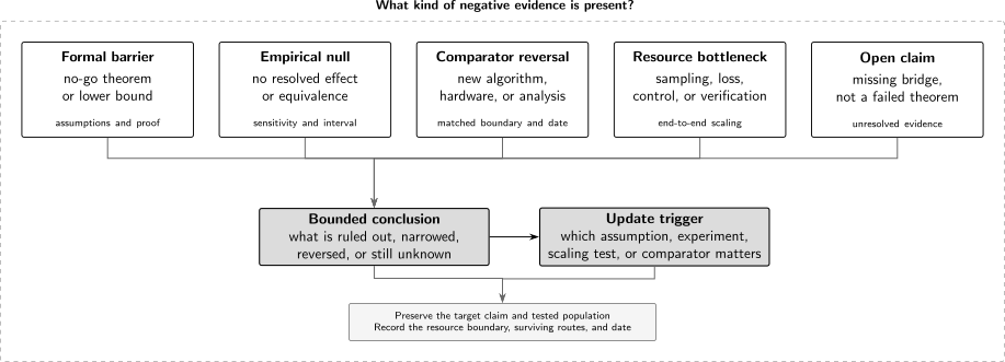
Negative evidence has several logical forms. A theorem inherits the scope of its assumptions; a null requires sensitivity or equivalence analysis; a benchmark reversal requires a matched and dated comparator; an overhead result requires an end-to-end resource boundary; and an open claim records a missing bridge rather than a failure. Each path should end in a bounded conclusion and an explicit update trigger.

The Limitation Record

For every entry, preserve:

Field	Question
target claim	what exact proposition is being limited?
result class	theorem, lower bound, null, equivalence, reversal, overhead, or open claim?
assumptions	access model, noise, locality, code family, data distribution, or apparatus regime?
tested population	which instances, devices, states, circuits, times, and scales?
sensitivity	which effect sizes or scaling laws could the study distinguish?
comparator	what baseline, version, hardware, and date?
resource boundary	which setup, samples, retries, control, verification, and infrastructure costs?
bounded conclusion	exactly what is ruled out, narrowed, or unsupported?
surviving routes	which regimes or alternative methods remain possible?
update trigger	what theorem, experiment, scaling study, or comparator would change the entry?

A useful record does not say “QAOA does not work” or “quantum sensing loses under noise.” It names the depth, instance family, noise model, estimator, and performance criterion for which the limitation was established.

Statistical Discipline for Null Results

Failure to reject is not equivalence

Let

$$\Delta = \theta_{\rm candidate} - \theta_{\rm baseline}$$

be the effect relevant to the claim. A conventional test may fail to reject $\Delta=0$. That does not establish $\Delta=0$.

Before collecting data, define a smallest effect $\Delta_{\min}>0$ that would matter scientifically or practically. Evidence of practical equivalence can be claimed when an appropriate confidence interval satisfies

$${\rm CI}_{1-\alpha}(\Delta) \subset \left[ -\Delta_{\min}, \Delta_{\min} \right].$$

Three outcomes are then distinct:

Interval position	Interpretation
entirely beyond the improvement margin	evidence for a meaningful improvement
entirely inside the equivalence interval	evidence that any difference is smaller than the chosen meaningful margin
overlaps meaningful improvement, equivalence, and harm	inconclusive at the achieved sensitivity

The margin must come from the task, not from the observed interval. Choosing it after seeing the data turns an equivalence analysis into another selection step.

State what the study could detect

A negative report should include:

• the target effect or scaling exponent;
• power or expected interval width under a prespecified model;
• the independent experimental unit;
• systematic and model uncertainty;
• stopping and exclusion rules;
• the tested parameter range;
• the strongest effect still compatible with the data.

For a benchmark over problem instances, the independent unit may be the instance, not the number of shots used to estimate each score. For hardware generalization, many shots on one device and one day do not replace multiple devices or calibration epochs.

Diagnose floor effects

A null can occur because both methods hit:

• a finite-shot noise floor;
• a detector or readout floor;
• a small-instance ceiling where every method succeeds;
• a time limit where no method converges;
• a verification floor that cannot distinguish outputs;
• a classical preprocessing bottleneck shared by both methods.

The correct conclusion may be “the experiment could not resolve the difference,” not “the methods are equal.”

End-to-End Bottlenecks

Amdahl’s law for quantum workflows

Suppose fraction $f$ of a baseline runtime can be accelerated by a quantum subroutine with segment speedup $S_q$, while the remaining fraction is unchanged. Under the simplest serial model, the total speedup is

$$S_{\rm total} = \frac{1}{ (1-f)+f/S_q }.$$

Even $S_q\to\infty$ gives

$$S_{\rm total} \leq \frac{1}{1-f}.$$

If state preparation, data movement, repeated measurements, decoding, verification, or output interpretation dominate, accelerating the coherent kernel does not establish an end-to-end advantage. Parallelism and overlap can modify this expression, but they must be scheduled rather than assumed.

Retries and acceptance

For statistically independent attempts with delivered-success probability $p_{\rm del}$ and mean attempt cost $T_{\rm att}$, the idealized expected time to one delivered result is

$$\mathbb E[T_{\rm del}] = \frac{T_{\rm att}}{p_{\rm del}}.$$

This exposes postselection, heralding, optimizer restarts, failed jobs, and probabilistic state preparation. A high conditional fidelity can coexist with poor time to solution when $p_{\rm del}$ is small.

Error-mitigation sampling

Many mitigation estimators combine noisy expectation estimates linearly:

$$\widehat\mu_{\rm mit} = \sum_j \eta_j\widehat\mu_j.$$

For independent estimates,

$$\operatorname{Var} \left( \widehat\mu_{\rm mit} \right) = \sum_j \eta_j^2 \operatorname{Var} \left( \widehat\mu_j \right).$$

Large positive and negative coefficients can cancel bias while amplifying variance. In probabilistic error cancellation, if $\gamma=\sum_j|\eta_j|$, a common shot-overhead scale is $\gamma^2$ relative to an unmitigated estimate, subject to allocation and protocol details. Fundamental bounds show that generic mitigation cannot arbitrarily erase accumulated noise at constant sampling cost.

Error mitigation can still be useful for selected observables and circuit regimes. The limitation is that improved bias, sampling overhead, residual model dependence, and total runtime must be reported together.

Error Mitigation Overview owns finite-regime method selection, explicit estimator accounting, combination rules, and held-out validation; this page retains durable lower-bound and no-go scope, benchmark reversals, and negative-result reporting.

Limits of Error Mitigation owns mitigation-specific theorem statements, finite resource stress tests, and local escalation decisions; this page retains the durable cross-domain ledger of no-go scope, empirical reversals, and update triggers.

Durable Limitation Ledger

Unstructured search has only a quadratic black-box speedup

Grover search gives $O(\sqrt N)$ oracle queries, and the Bennett–Bernstein– Brassard–Vazirani lower bound shows that this scaling is optimal for unstructured black-box search. Encoding every optimization problem as a marked-item search therefore does not create an exponential speedup.

What it rules out: a better generic query scaling when the oracle hides all structure.

What remains open: algorithms that exploit group structure, algebraic promises, geometry, sparsity, or problem-specific distributions.

Shallow QAOA has instance-dependent reachability limits

Fixed-depth QAOA is local on bounded-degree problem graphs. Results on reachability deficits, symmetry protection, and specific graph families show that shallow circuits can fail to reach high-quality regions even without hardware noise. Classical local algorithms can match or outperform low-depth QAOA in some settings. The canonical QAOA page owns the ansatz, hypotheses, guarantees, and resource model; this page retains the cross-study limitation record and update triggers.

These are targeted results, not a universal theorem against QAOA. Increasing depth changes what the circuit can see, while also increasing optimization, sampling, compilation, and noise costs. A practical advantage claim therefore needs a scaling comparison among solution quality, depth, training cost, and current classical methods.

Current bounded conclusion: low-depth QAOA has no established generic practical speedup for combinatorial optimization.

Update trigger: a prespecified instance family on which end-to-end, verified quality–cost scaling beats competitive classical methods.

Variational trainability can become exponentially expensive

Random, sufficiently expressive parameterized circuits can exhibit barren plateaus in which gradient variance decreases exponentially with system size. Global costs, deep random ansatzes, entanglement structure, symmetries, and noise create distinct mechanisms. Under local Pauli noise, work in 2021 proved noise-induced gradient suppression that is exponential in depth and therefore in system size when depth grows linearly.

That result has assumptions. In 2026, analysis of local non-unital noise found that local-observable costs need not exhibit the same barren plateau. However, the same noise made typical circuits effectively shallow and enabled efficient classical estimation in the studied average-case setting. Removing one trainability symptom did not automatically restore quantum advantage.

Problem-inspired ansatzes, local costs, initialization, symmetry sectors, adaptive growth, error correction, and engineered dissipation can change the picture. Their success should be established by gradient signal-to-noise, shots, optimizer calls, final quality, and scaling across held-out instances.

Current bounded conclusion: trainability is not guaranteed by a shallow finite-size demonstration, and generic noisy VQA speedup remains unestablished.

Classical data can erase an apparent quantum-learning separation

Quantum Machine Learning proposals can assume amplitude-encoded inputs or sample-and-query access that hides substantial data preparation. Tang’s quantum-inspired recommendation algorithm showed that, under a classical sampling access model analogous to the quantum input assumption, a previously claimed exponential separation did not survive.

The QML owner specifies the exact access and learning hypotheses plus positive guarantees; this page retains the durable limitation and update ledger.

Separately, the “power of data” analysis showed that classical learners can predict labels from examples even when independently computing the underlying quantum process is hard. Hard simulation does not imply hard supervised learning.

What it rules out: inferring prediction advantage solely from the classical hardness of simulating the feature-generating circuit.

What remains open: quantum-native data, carefully separated access models, tasks with provable learning separations, and practical data sets on which matched classical learners are beaten.

Classical simulation can move the advantage frontier

A 2023 127-qubit kicked-Ising experiment reported quantum results beyond the then-used classical approximations in a strongly entangled regime. In 2024, Tindall and collaborators used geometry-aware tensor-network belief propagation to produce more accurate and precise classical results for that experiment, while Begušić and collaborators developed another fast, converged classical simulation.

The quantum measurements did not cease to exist. The comparative interpretation changed because the classical frontier moved. The episode also yielded useful algorithmic insight: hardware geometry, observable locality, entanglement structure, and approximation error mattered more than qubit count alone.

Current bounded conclusion: a disagreement with selected classical approximations is not durable evidence of utility or advantage without adversarial classical follow-up.

Update trigger: a task with verified quantum output, a dated broad classical search, matched resources, and a separation robust to new simulation methods.

Generic exponential advantage in ground-state chemistry is not established

Quantum phase estimation has rigorous advantages for some Hamiltonian and access models, and fault-tolerant chemistry resource estimates can be valuable. A stronger claim is that chemically typical ground states are both efficiently preparable on a quantum computer and generically exponentially hard for the best classical heuristics at chemically relevant accuracy.

Lee and collaborators examined evidence for that hypothesis and found that it was not established by the tested families and diagnostics. “Generic chemistry” is itself difficult to define, state preparation can be hard on both quantum and classical computers, and classical electronic-structure methods exploit locality, weak correlation, tensor structure, and chemical priors.

What it does not rule out: polynomial or high-degree speedups, special strongly correlated families, dynamics, response properties, or future algorithms with validated state preparation.

Current bounded conclusion: exponential quantum advantage should not be treated as a generic property of ground-state quantum chemistry.

Error mitigation cannot replace scalable error correction at fixed cost

Error mitigation estimates ideal quantities from noisy executions without maintaining a protected logical state. It can reduce bias in useful finite regimes. General bounds connect the achievable error reduction to sampling overhead, circuit noise, and distinguishability lost to the environment. Later bounds tightened exponential overhead statements for broad circuit and noise settings.

What it rules out: assuming that arbitrarily deep noisy computation can be made ideal with constant sampling and no additional model assumptions.

What remains open: problem-specific observables, shallow circuits, symmetry verification, virtual distillation, learned noise structure, and hybrids in which mitigation supplements rather than replaces QEC.

The symmetry-verification specialist owns finite sector-filtering licenses, invisible-error boundaries, acceptance cost, and abstention; this page retains the broader scoped limitation ledger.

Fault tolerance has structural overhead, not only better components

The Eastin–Knill theorem means an ordinary exact code cannot obtain a universal logical unitary set entirely from transversal gates. Magic-state distillation, code switching, gauge fixing, lattice surgery, or related machinery supplies the missing operations at a cost.

For two-dimensional geometrically local commuting codes, the Bravyi–Poulin– Terhal tradeoff constrains encoded rate and distance:

$$k d^2 \leq c n,$$

where $n$ is the number of physical subsystems, $k$ the number of encoded qubits, $d$ the distance, and $c$ depends on locality details. The theorem does not apply unchanged to every nonlocal, subsystem, dynamical, or higher- dimensional construction.

Threshold behavior addresses suppression of logical faults with increasing code size. It does not erase factories, routing, measurement, reset, decoder latency, leakage handling, or rare correlated events. Error-Correction Case Studies gives the experimental evidence ladder.

Current bounded conclusion: better physical error rates and a below- threshold memory are necessary evidence, not a complete low-overhead fault-tolerant computer.

Noise often restores standard-quantum-limit scaling

Ideal entangled probes can attain Heisenberg-like scaling in selected noiseless models. For independent Markovian dephasing in frequency estimation, Huelga and collaborators showed that the asymptotic scaling advantage can disappear. Broader channel bounds show that dephasing, depolarization, spontaneous emission, and loss generically reduce the asymptotic gain to a constant factor in common models.

This does not say entanglement is useless. Constant gains can be valuable, and ancillas, temporal correlations, error correction, non-Markovian structure, adaptive protocols, or a different resource count can change a bound.

Current bounded conclusion: a squeezed or entangled probe does not by itself establish Heisenberg scaling or end-to-end sensor advantage under realistic loss and noise.

Pure loss imposes a repeaterless rate–distance limit

For a pure-loss bosonic channel with transmissivity $\eta$, the two-way-assisted secret-key capacity without quantum repeaters is

$$K(\eta) = -\log_2(1-\eta).$$

At high loss,

$$K(\eta) \simeq \frac{\eta}{\ln 2}.$$

This Pirandola–Laurenza–Ottaviani–Banchi bound is a fundamental benchmark per channel use under its point-to-point model. Better detectors and coding can approach the bound but cannot change its high-loss scaling. Surpassing that direct-transmission scaling requires changing the architecture, for example with repeater nodes, memories, or a protocol whose channel partition is explicitly different.

What it does not rule out: trusted relays, satellite geometry, twin-field architectures with an intermediate measurement station, or genuine quantum repeaters. Those systems must be compared under their own trust and resource boundaries.

Open Claims Are Not Negative Results

Several important propositions remain neither proved nor refuted:

• a practical quantum advantage for a valuable optimization workload;
• broad quantum-learning advantage on classical industry data;
• economical fault-tolerant chemistry at a useful accuracy and turnaround time;
• a scalable universal architecture with acceptable energy, control, and manufacturing overhead;
• network services that beat direct architectures after memories, scheduling, and availability are included;
• metrological advantage that survives full instrument overhead across a valuable operating range.

Label these open, not failed. Absence of a convincing demonstration is not a no-go theorem. Conversely, commercial activity, investment, and roadmaps are not evidence that the claim has already been established.

An open-claim record should name the missing bridge. “More research is needed” is too vague. Examples include:

• no matched classical baseline at useful instance size;
• no verified output beyond tractable instances;
• no scaling across code distance;
• no unconditional rate after postselection;
• no end-to-end resource estimate;
• no holdout test on representative data;
• no manufacturing or calibration yield evidence.

How to Report a Negative Result

Preserve the planned test

Report the original hypothesis, primary endpoint, smallest meaningful effect, sample-size rationale, stopping rule, and exclusions. Distinguish prespecified, secondary, and exploratory analyses.

Show raw and normalized views

Provide:

• per-instance or per-device results, not only an average;
• uncertainty intervals and distribution tails;
• conditional and unconditional performance;
• per-cycle and per-time quantities where both matter;
• component and end-to-end resource views;
• chronological plots when drift or rare events matter.

Report implementation competence

A negative comparison against a poorly tuned candidate is weak evidence about the method. Record:

• hyperparameter and compiler search;
• convergence diagnostics;
• calibration validity;
• classical and quantum implementation checks;
• positive controls known to succeed;
• ablations that locate the bottleneck.

This does not require unlimited tuning. It requires a fair, declared budget and evidence that the implementation exercised the intended mechanism.

Separate local failure from family-wide failure

Use language such as:

Under noise model $\mathcal N$, depth scaling $L(n)$, observable family $\mathcal O$, and the tested parameter distribution, the gradient signal fell below the declared resolvability threshold. This rules out the tested training protocol at the measured shot budget; it does not rule out all structured ansatzes or fault-tolerant implementations.

The boundary is part of the result, not a disclaimer added afterward.

Archive the reversal

When a comparator overtakes a result, retain both records:

1. what was supported at the original date;
2. which new algorithm, hardware, or analysis changed the comparison;
3. whether the original output remains valid;
4. which broader claim must be withdrawn or narrowed;
5. the new baseline and update date.

This makes scientific progress visible rather than rewriting history.

What Changes a Limitation Entry?

Entry type	Strong update
no-go theorem	relax an assumption, prove a stronger theorem, or exhibit a valid counterexample outside the old scope
lower bound	change the access model or prove a tighter matching algorithm
empirical null	improve sensitivity, broaden the population, or replicate under a stronger design
benchmark reversal	produce a new matched result against the updated frontier
overhead bottleneck	demonstrate improved scaling or move the bottleneck end to end
open claim	supply the named missing bridge with verification and uncertainty

A larger device count is not automatically the relevant update. If the limitation is data loading, loss, verification, or a classical baseline, more qubits may leave the claim unchanged.

Common Mistakes

• Treating $p>0.05$ as evidence of no effect.
• Calling an underpowered experiment an equivalence result.
• Turning one adverse instance family into a theorem about all algorithms.
• Omitting the assumptions of a no-go theorem.
• Treating a later classical simulation as proof that the quantum experiment was fraudulent or scientifically worthless.
• Preserving an obsolete advantage headline after its comparator was beaten.
• Reporting the coherent-kernel speedup while excluding dominant workflow stages.
• Calling sampling overhead a small constant without showing how it scales.
• Treating a finite-size crossover as asymptotic evidence.
• Calling an unproved application claim false merely because it remains open.
• Hiding negative seeds, devices, instances, or calibration windows.
• Publishing only the failed endpoint without diagnostics of implementation competence.
• Describing structural overhead as an engineering detail that can be assumed away.
• Letting “quantum-inspired” or “classically simulable” substitute for a matched resource comparison.

Exercises

1. Null or equivalence?

A measured speed difference is $\widehat\Delta=0.8\%$ with a $95\%$ confidence interval $[-2.5\%,4.1\%]$. The prespecified practically meaningful margin is $\Delta_{\min}=1\%$. What can be concluded?

Solution

The interval contains zero, so the study does not show a statistically resolved difference under the chosen procedure. It also extends well outside the equivalence interval $[-1\%,1\%]$, so it does not show practical equivalence.

The correct disposition is inconclusive at the achieved sensitivity. Effects ranging from a modest harm to a meaningful improvement remain compatible with the interval.

2. Apply Amdahl’s law

A quantum kernel occupies $f=0.20$ of the baseline end-to-end runtime and is accelerated by a factor $S_q=100$. Compute the idealized total speedup and its maximum as $S_q\to\infty$.

Solution

The total speedup is

$$S_{\rm total} = \frac{1}{0.80+0.20/100} \approx 1.247.$$

Even an infinitely fast kernel gives

$$S_{\rm total}^{\max} = \frac{1}{0.80} = 1.25.$$

The hundredfold segment improvement supports a component claim, while the workflow can improve by at most $25\%$ under this serial resource model.

3. Include retry overhead

A heralded protocol takes $4\ {\rm ms}$ per attempt and delivers a useful output with probability $2\times10^{-3}$. Estimate the idealized mean time per delivered output.

Solution

Using the geometric-attempt model,

$$\mathbb E[T_{\rm del}] = \frac{4\times10^{-3}\ {\rm s}} {2\times10^{-3}} = 2\ {\rm s}.$$

A conditional operation time of $4\ {\rm ms}$ is therefore not a $4\ {\rm ms}$ delivered-service latency. Queueing, timeout, reset, and latency-tail effects could make the operational value larger.

4. Estimate mitigation variance

An estimator is

$$\widehat\mu_{\rm mit} = 1.5\widehat\mu_1 - 0.5\widehat\mu_2.$$

The two independent unmitigated estimates each have variance $\sigma^2/N$. Find the mitigated variance and compare it with one unmitigated estimate using the same $N$ for each circuit.

Solution

Independence gives

$$\operatorname{Var} \left( \widehat\mu_{\rm mit} \right) = \left( 1.5^2+0.5^2 \right) \frac{\sigma^2}{N} = 2.5\frac{\sigma^2}{N}.$$

The variance is $2.5$ times that of one unmitigated estimate, and the protocol also used $2N$ total shots. Whether the comparison should fix shots, elapsed time, or precision depends on the claim. Bias reduction must be compared with this variance and execution cost.

5. Scope a no-go theorem

Someone summarizes Eastin–Knill as “fault-tolerant universal gates are impossible.” Repair the statement and name two surviving routes.

Solution

The theorem rules out a universal set of transversal encoded unitaries for a nontrivial exact finite-dimensional code that detects arbitrary errors on each physical subsystem. It does not rule out universal fault-tolerant computation.

Surviving routes include magic-state injection and distillation, code switching, gauge fixing, teleportation-based gates, lattice surgery, and approximate or otherwise out-of-scope constructions. Any two suffice, with their own error and overhead analysis.

6. Interpret a classical reversal

A quantum experiment accurately measured an observable in 2023 and compared it with the best classical approximations used in that paper. A new classical algorithm reproduces the observable more accurately and faster in 2024. Which claims change?

Solution

The validity of the 2023 measured data does not change merely because the classical algorithm improved. Claims tied to those observations and their uncertainty can remain supported.

The comparative claim that the observable lay beyond practical classical calculation, or that the experiment established utility or advantage against the classical frontier, must be updated. The record should identify the old baseline, the new algorithm and date, and whether any narrower hardware or physics conclusion remains.

7. Bound a direct optical link

A pure-loss link has transmissivity $\eta=10^{-4}$. Estimate its high-loss PLOB capacity in secret bits per channel use. Does a protocol below this rate disprove quantum repeaters?

Solution

At high loss,

$$K(\eta) \simeq \frac{10^{-4}}{\ln2} \approx 1.44\times10^{-4}$$

secret bits per channel use.

A protocol below this rate does not disprove repeaters. The PLOB value is the ultimate repeaterless benchmark in the stated channel model. A repeater protocol may be immature, suffer local inefficiencies, or optimize another resource. Evidence for a repeater advantage requires an end-to-end comparison that eventually surpasses the appropriate direct bound under matched channel uses and trust assumptions.

8. Classify an open claim

No published experiment has shown an end-to-end practical quantum advantage for a valuable logistics workload under a current classical baseline. Is the claim “quantum optimization will never be useful” supported?

Solution

No. The available statement is that practical advantage for the declared workload remains unestablished. Absence of a demonstration does not prove future impossibility.

A useful ledger entry names the missing bridge: representative instances, matched quality and time to solution, competitive classical methods, verification, all tuning and retry costs, and scaling beyond a favorable finite-size point. A theorem or broad empirical program would be needed for a stronger negative conclusion.

References

1. National Academies of Sciences, Engineering, and Medicine, Quantum Computing: Progress and Prospects (National Academies Press, 2019), doi:10.17226/25196.
2. C. H. Bennett, E. Bernstein, G. Brassard, and U. Vazirani, “Strengths and weaknesses of quantum computing,” SIAM Journal on Computing 26, 1510–1523 (1997), doi:10.1137/S0097539796300933.
3. L. K. Grover, “A fast quantum mechanical algorithm for database search,” in Proceedings of the 28th Annual ACM Symposium on Theory of Computing, 212–219 (1996), doi:10.1145/237814.237866.
4. J. R. McClean et al., “Barren plateaus in quantum neural network training landscapes,” Nature Communications 9, 4812 (2018), doi:10.1038/s41467-018-07090-4.
5. M. Cerezo et al., “Cost function dependent barren plateaus in shallow parametrized quantum circuits,” Nature Communications 12, 1791 (2021), doi:10.1038/s41467-021-21728-w.
6. S. Wang et al., “Noise-induced barren plateaus in variational quantum algorithms,” Nature Communications 12, 6961 (2021), doi:10.1038/s41467-021-27045-6.
7. A. A. Mele et al., “Noise-induced shallow circuits and the absence of barren plateaus,” Nature Physics 22, 751–756 (2026), doi:10.1038/s41567-026-03245-z.
8. V. Akshay, H. Philathong, M. E. S. Morales, and J. Biamonte, “Reachability deficits in quantum approximate optimization,” Physical Review Letters 124, 090504 (2020), doi:10.1103/PhysRevLett.124.090504.
9. M. B. Hastings, “Classical and quantum bounded depth approximation algorithms,” Quantum Information and Computation 19, 1116–1140 (2019), doi:10.26421/QIC19.13-14-3.
10. E. Tang, “A quantum-inspired classical algorithm for recommendation systems,” in Proceedings of the 51st Annual ACM SIGACT Symposium on Theory of Computing, 217–228 (2019), doi:10.1145/3313276.3316310.
11. H.-Y. Huang et al., “Power of data in quantum machine learning,” Nature Communications 12, 2631 (2021), doi:10.1038/s41467-021-22539-9.
12. R. Takagi, S. Endo, S. Minagawa, and M. Gu, “Fundamental limits of quantum error mitigation,” npj Quantum Information 8, 114 (2022), doi:10.1038/s41534-022-00618-z.
13. Y. Quek et al., “Exponentially tighter bounds on limitations of quantum error mitigation,” Nature Physics 20, 1648–1658 (2024), doi:10.1038/s41567-024-02536-7.
14. Y. Kim et al., “Evidence for the utility of quantum computing before fault tolerance,” Nature 618, 500–505 (2023), doi:10.1038/s41586-023-06096-3.
15. J. Tindall, M. Fishman, E. M. Stoudenmire, and D. Sels, “Efficient tensor network simulation of IBM’s Eagle kicked Ising experiment,” PRX Quantum 5, 010308 (2024), doi:10.1103/PRXQuantum.5.010308.
16. T. Begušić, J. Gray, and G. K.-L. Chan, “Fast and converged classical simulations of evidence for the utility of quantum computing before fault tolerance,” Science Advances 10, eadk4321 (2024), doi:10.1126/sciadv.adk4321.
17. S. Lee et al., “Evaluating the evidence for exponential quantum advantage in ground-state quantum chemistry,” Nature Communications 14, 1952 (2023), doi:10.1038/s41467-023-37587-6.
18. S. F. Huelga et al., “Improvement of frequency standards with quantum entanglement,” Physical Review Letters 79, 3865–3868 (1997), doi:10.1103/PhysRevLett.79.3865.
19. R. Demkowicz-Dobrzański, J. Kołodyński, and M. Guţă, “The elusive Heisenberg limit in quantum-enhanced metrology,” Nature Communications 3, 1063 (2012), doi:10.1038/ncomms2067.
20. S. Pirandola et al., “Fundamental limits of repeaterless quantum communications,” Nature Communications 8, 15043 (2017), doi:10.1038/ncomms15043.
21. B. Eastin and E. Knill, “Restrictions on transversal encoded quantum gate sets,” Physical Review Letters 102, 110502 (2009), doi:10.1103/PhysRevLett.102.110502.
22. S. Bravyi, D. Poulin, and B. Terhal, “Tradeoffs for reliable quantum information storage in 2D systems,” Physical Review Letters 104, 050503 (2010), doi:10.1103/PhysRevLett.104.050503.
23. S. Bravyi and R. König, “Classification of topologically protected gates for local stabilizer codes,” Physical Review Letters 110, 170503 (2013), doi:10.1103/PhysRevLett.110.170503.
24. C. Gidney and M. Ekerå, “How to factor 2048 bit RSA integers in 8 hours using 20 million noisy qubits,” Quantum 5, 433 (2021), doi:10.22331/q-2021-04-15-433.
25. T. Hoefler, T. Häner, and M. Troyer, “Disentangling hype from practicality: on realistically achieving quantum advantage,” Communications of the ACM 66, 82–87 (2023), doi:10.1145/3571725.
26. D. Lakens, “Equivalence tests: a practical primer for t tests, correlations, and meta-analyses,” Social Psychological and Personality Science 8, 355–362 (2017), doi:10.1177/1948550617697177.

Further Connections

• Verification of Quantum Advantage supplies the positive evidence chain and adversarial classical challenge.
• Variational Quantum Algorithms owns ansatz design, gradient estimation, barren-plateau mechanisms, noise, and optimizer validation.
• Resource Estimation Tools turns overhead claims into versioned scenarios and sensitivity analyses.
• Tensor-Network Simulation develops the classical methods behind several moving-frontier examples.
• Sensing Case Studies compares quantum enhancement under matched bandwidth, loss, spatial resolution, calibration, and uncertainty.
• Network Case Studies separates direct-link bounds, repeater-enabling components, and delivered network services.