Quantum Machine Learning

Quantum machine learning is a collection of learning problems and model families, not one algorithm. Quantum processors can supply feature spaces, variational predictors, sample generators, or coherent processing of quantum examples, and rigorous separations exist under explicit access and hardness assumptions. None of those facts alone establishes a generic end-to-end advantage on ordinary classical data. A meaningful claim must first fix the task, data type, access interface, statistical protocol, requested output, resource boundary, classical comparator, and strength of evidence. This page develops that discipline while distinguishing representation hardness, trainability, generalization, sampling hardness, and practical advantage.

Required background. Algorithmic Primitives supplies access, error, and output conventions; Variational Quantum Algorithms supplies the generic hybrid loop and gradient-estimation framework; and Random Variables supplies distributions, expectations, and iid sampling.

Helpful background. Classical Information Review owns the general representation-and-total-cost comparator; Quantum Oracles owns coherent black-box semantics; Algorithmic Benchmarking owns the generic benchmark protocol; and Verification of Quantum Advantage owns adversarial tests of advantage claims.

Quantum Learning as a Statistical Input–Output Task

Let $\mathcal D$ be a distribution on examples $(X,Y)\in\mathcal X\times \mathcal Y$. A supervised learner receives a training sample, applies a declared procedure to a hypothesis family $\mathcal H$, and returns a predictor $h$. Its quality is defined only after choosing a loss $\ell(h(x),y)$ and an output contract. A binary classifier might return a label, a score, or a calibrated class probability; those outputs support different uses and cannot be scored as if they were interchangeable.

The same care applies beyond classification. Regression returns a number or interval; density estimation seeks evaluable probabilities or a density representation; generative modeling may promise only samples; property prediction for quantum systems may return expectation values for a specified observable family. A procedure that samples from $q$ need not evaluate $q(z)$, and a state-preparation circuit need not reveal a classical description of its state. The requested output can decide whether a proposed quantum saving survives readout.

The statistical protocol has three roles. Training data determine parameters. Validation data select feature scaling, representation, architecture, regularization, optimizer, checkpoint, threshold, mitigation, or any other pipeline choice. A held-out test sample is touched once, after the complete pipeline is frozen. Changing a choice after inspecting test performance turns that test set into selection data; a new independent test set is then needed.

The survey by Biamonte et al. (2017) organizes many quantum-assisted learning proposals, but the label “QML” supplies no shared complexity statement. A kernel method, a variational circuit, a Born sampler, and a learner acting on unknown quantum states differ in input, operations, output, and cost. The durable unit of analysis is a fully specified statistical input–output problem, not the technology named in its title.

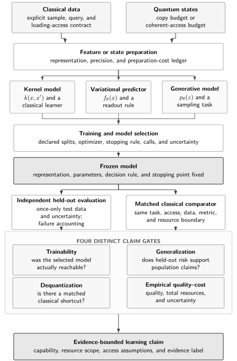
Classical data require an explicit loading contract, while quantum inputs require a copy or coherent-access budget. Training and selection followed by independent validation belong to the executable algorithm. Qubit width is not loading time, and generalization, trainability, dequantization, and empirical quality–cost are distinct audit gates.

The Ten-Field Quantum-Learning Claim Record

The following record instantiates the chapter-wide ten-field contract for a binary classifier on explicitly stored real vectors. It is deliberately concrete: dimension, split sizes, loader, and selection budget are part of the claim. It specifies a family to be tested, not a promise of advantage.

Field	Required declaration
Problem family and size	Binary supervised classification of $d$-component real vectors, with prespecified training, validation, and test counts $m_{\rm tr}$, $m_{\rm val}$, and $m_{\rm te}$.
Promise and instance distribution	Name the data source, inclusion rules, label definition, class balance, feature dimension, sampling unit, distribution $\mathcal D$, and seeded split rule; prevent related records from crossing splits.
Access and encoding	Inputs are explicit classical arrays; feature scaling is fitted on training data; a documented circuit $U_\phi(x)$ loads each vector, including loader construction, precision, depth, and memory cost.
Output and use	Return $f_\theta(x)\in[-1,1]$, the frozen thresholded label with a declared tie rule, and, only if calibrated, a probability used for the stated decision.
Success and error	Optimize a bounded training loss; select by a prespecified validation metric and budget; report fresh-test risk, uncertainty, calibration, and absolute as well as comparative metrics.
Algorithmic idea	Encode $x$ as $\rho(x)$, apply a declared variational circuit, and estimate a bounded observable whose expectation is the classification score.
Executable procedure	Archive preprocessing, circuits, optimizer, data order, seeds, shot allocation, stopping and checkpoint rules, threshold selection, mitigation, frozen inference, and the once-only test evaluation.
Resource ledger	Count loader and memory construction, preprocessing, every circuit and shot, compiled gates and depth, classical optimization and search, communication, failures, mitigation, decoding, and wall-clock time.
Classical comparator	Give simple, strong, and task-specialized classical models the same raw data, splits, selection budget, metric, and total-cost boundary; add matched strong-access or dequantized comparators where relevant.
Evidence and limits	Bound the conclusion to the named distribution, sizes, representation, access, devices or simulator, noise, comparator portfolio, and confidence interval; do not infer generic advantage.

The record separates the learned object from the procedure that selected it. A final two-qubit circuit does not disclose how many candidate feature maps, optimizers, seeds, checkpoints, or mitigation settings were tried. Nor does a high test accuracy disclose loading time or the performance of a tuned classical portfolio. The Claims and Evidence Checklist helps turn this record into a publication-level claim.

Classical Data, Quantum Data, and Access Models

An access interface is a mathematical or physical resource. Granting it as an oracle can support a valid conditional theorem, but does not implement the interface for free. The table fixes six common interfaces before comparing complexities.

Interface	Object supplied	Allowed operations	Construction or acquisition cost	Comparison boundary
Classical explicit data	Stored feature array and labels	Read, index, preprocess, copy, and communicate ordinary records	Data collection, storage, parsing, indexing, and preprocessing are charged	Compare with algorithms receiving the same explicit records and account for input-reading cost
Sample access	Distribution or data stream	Draw iid examples; sample-and-query variants additionally sample indices and query entries or norms	Sampling instrument, database, normalization metadata, latency, and repeated draws are charged	Do not silently upgrade iid samples to arbitrary coherent queries or full-table access
Coherent value or feature oracle	Reversible map such as $O_x\lvert j,b\rangle=\lvert j,b\oplus x_j\rangle$	Query in superposition and, when declared, call the inverse	Reversible memory, precision, loader synthesis, routing, and communication are charged or explicitly assumed	Compare conditional query counts separately from end-to-end implementation cost
Amplitude-prepared state	Copies of $\lvert x\rangle=\lVert x\rVert^{-1}\sum_jx_j\lvert j\rangle$ or access to its preparation unitary	Measure copies; coherent-unitary access may permit $U_x$ and $U_x^\dagger$	Normalization, exact or approximate state preparation, copies, and memory are charged	Match approximation and give classical comparators analogous sample-and-query access when appropriate
Quantum-state copies	Independent systems in unknown states $\rho_x$	Apply allowed single-copy or joint measurements and classical postprocessing	Experimental preparation, transmission, storage, destructive measurements, and lost copies are charged	No-cloning forbids treating a consumed unknown state as reusable classical data
Circuit-generated quantum data	A known or black-box preparation process	Execute the circuit, perhaps coherently with its inverse, then measure specified observables	Circuit construction, control, depth, noise, reset, calibration, and executions are charged	Distinguish a circuit description, executable access, stored states, and classical measurement records

Classical examples and coherent access

An explicit array supports arbitrary classical inspection after storage. Iid sample access supplies fresh examples but not necessarily random entry queries. Sample-and-query access is stronger: typical formulations allow sampling an index proportional to squared magnitude and querying entries or norms. A qRAM-style lookup or reversible feature oracle is stronger again, because it preserves superpositions and must be synthesized or assumed. A state-preparation circuit adds its own approximation and gate model.

These distinctions determine what a complexity result means. A query theorem may count calls to $O_x$ while intentionally excluding its engineering; an end-to-end claim may not. Classical preprocessing can be amortized over many training runs or predictions, but only a declared number of uses justifies that division. Data collection and communication remain outside neither method merely because the final circuit is short.

Quantum examples, copies, and measurement budgets

Quantum data may arrive as independent copies of unknown states, coherent access to a preparation unitary and its inverse, a quantum memory retaining systems, or a circuit generating fresh states. These are inequivalent. Unknown states cannot be cloned, and a destructive measurement consumes its copy. Joint measurements across retained systems can be more powerful than separate measurements, but require corresponding memory and control. Classical measurement records discard capabilities of the original states.

Huang, Kueng, and Preskill (2021) prove access-sensitive information-theoretic statements for predicting quantum experiments: average prediction and uniformly accurate prediction over all inputs can have very different copy complexity. A coherent-quantum-data result therefore does not automatically apply to a conventional table.

Construction, amortization, and fair comparison

Every comparison should expose construction, loading, memory, communication, and amortization. If a database costs $C_{\rm build}$ to convert into a reversible loader, each invocation costs $C_{\rm call}$, and it is used $A$ times, reporting only $C_{\rm call}$ hides $C_{\rm build}/A$ per use. The same logic applies to a fitted classical index, calibration data, and experimental state preparation. Different boundaries can be informative, but they must be displayed side by side rather than mixed.

An $N$-component amplitude vector fits into $\lceil\log_2N\rceil$ qubits, yet the generic normalized vector has $O(N)$ independent real parameters. Exact arbitrary state synthesis therefore has correspondingly large description and gate cost Shende, Bullock, and Markov (2006). Efficient preparation is possible for declared structure. Grover and Rudolph (2002), for example, give a construction for efficiently integrable distributions. Such a family or an oracle assumption is a useful exception, not evidence for generic logarithmic loading.

Encoding Classical Features into Quantum States

A density-operator feature map prepares

$$\rho(x)=U_\phi(x)\lvert0^n\rangle\!\langle0^n\rvert U_\phi^\dagger(x).$$

The encoding specifies which distinctions in the raw data become easy for a later measurement to detect. It is part of the model and must be fitted or chosen using training and validation data only.

Basis, angle, and amplitude encodings

Basis encoding maps discrete features to computational-basis strings. It can use one qubit per bit and shallow preparation, but continuous values require a declared quantization. Angle encoding maps features into rotations, such as $R_y(x_j)$ on qubit $j$; width is usually linear in features loaded in parallel, while repeated data re-uploading trades width for depth. Pérez-Salinas et al. (2020) show how repeated encodings and trainable one-qubit rotations can form a universal classifier family, a representation result rather than a training or advantage guarantee.

Amplitude encoding uses $\log_2N$ qubits for $N$ amplitudes, but pays the state-preparation cost just discussed. Re-uploading and entangling maps can generate rich Fourier spectra or nonlocal features, at the price of calls, precision, depth, and possible simulability changes. A comparison records width, loader gates and depth, approximation error, feature locality, sensitivity to rescaling, and classical simulation cost. “Fewer qubits” and “loads faster” are separate conclusions.

Feature maps are not free data loaders

A deliberately classically hard feature state can still be poorly aligned with labels. Expressivity asks how intricate a representation family is; task alignment asks whether its accessible geometry reflects the target. Increasing entanglement can make state simulation harder while making measured similarities nearly constant. Conversely, a simple local feature may solve the task.

The procedure must separate data acquisition, preprocessing, loader construction, state preparation, and model evaluation. If feature-map parameters are selected, their search is training cost. If a classical projection precedes the circuit, its fitting and inference belong in the ledger. Havlíček et al. (2019) constructed and implemented supervised feature-space models whose evidence combines a proposed hard map with finite experiments; those evidential layers should remain distinct.

Quantum Kernels and Feature-Space Models

Kernel methods separate quantum feature acquisition from a classical learner. The quantum device estimates similarities; a classical kernel algorithm fits coefficients, regularization, and threshold. This split can make the fitting problem convex while leaving feature acquisition statistically or computationally expensive.

State-overlap kernels and Gram matrices

For density-operator features, define the Hilbert–Schmidt overlap

$$k_F(x,x')=\operatorname{Tr}[\rho(x)\rho(x')].$$

For mixed states this is not the general Uhlmann fidelity. Only when both features are pure, $\rho(x)=\lvert\phi(x)\rangle\!\langle\phi(x)\rvert$, may one rewrite it as

$$k_F(x,x')= \lvert\langle\phi(x)\vert\phi(x')\rangle\rvert^2.$$

The ideal Gram matrix $K_{ij}=k_F(x_i,x_j)$ is Hermitian and positive semidefinite. For arbitrary complex coefficients $c_i$, set $A=\sum_i c_i\rho(x_i)$. Then

$$\sum_{i,j}c_i^*c_jK_{ij} =\operatorname{Tr}(A^\dagger A)\ge0.$$

This proof does not depend on a training algorithm. It also explains why a matrix of independently noisy overlap estimates can violate a property that the exact kernel must satisfy.

A SWAP test gives ancilla-zero probability

$$p_0=\frac{1+k_F}{2}, \qquad \widehat k_F=2\widehat p_0-1.$$

With $S$ independent ancilla measurements, Hoeffding’s inequality gives the conservative entrywise statement

$$\Pr\!\left(\lvert\widehat k_F-k_F\rvert\ge\epsilon\right) \le2\exp\!\left(-\frac{S\epsilon^2}{2}\right).$$

The relation between quantum encodings and reproducing-kernel feature spaces is developed by Schuld and Killoran (2019). The mathematical kernel guarantee is exact; efficient acquisition and usefulness for a label distribution require additional arguments.

Finite-shot kernels, regularization, and prediction

An $m$-example symmetric training Gram matrix has $m(m+1)/2$ distinct entries before shot repetitions. A validation set of size $v$ adds $vm$ cross-kernel entries, and testing adds more. Report allocation per entry, simultaneous uncertainty when many entries are used, and whether every comparator receives the same estimated matrix. Symmetrizing $\widehat K$, projecting negative eigenvalues away, adding a diagonal ridge, or changing kernel bandwidth can stabilize training, but each is a selected preprocessing choice and can alter the predictor.

One response to poorly resolved global overlaps is a projected quantum kernel,

$$k_{\mathrm{PQ}}(x,x') = \exp\!\left[ -\gamma\sum_{q=1}^{n} \lVert\rho_q(x)-\rho_q(x')\rVert_F^2 \right], \qquad \gamma>0,$$

where each $\rho_q$ is a declared reduced density operator. Local projections can improve resolvability while discarding nonlocal signal. In particular regimes, Thanasilp et al. (2024) prove exponential kernel concentration under hypotheses involving expressivity, entanglement, global measurements, or noise. That conditional result is not a theorem that every feature map and dataset concentrates. Geometry, estimation precision, regularization, and test performance must all be checked for the task.

Variational Quantum Classifiers

A variational classifier places a trainable channel after, or partly within, the feature map. Write

$$\rho_\theta(x)=V(\theta)\rho(x)V^\dagger(\theta), \qquad f_\theta(x)=\operatorname{Tr}[M\rho_\theta(x)], \qquad -I\preceq M\preceq I.$$

The operator bound ensures $f_\theta(x)\in[-1,1]$. It also turns the score into a legitimate two-outcome measurement model rather than an arbitrary number emitted by a circuit.

Observable scores and two-outcome decisions

For $y\in\{-1,+1\}$, define

$$E_y=\frac{I+yM}{2}, \qquad p_\theta(y\mid x)=\frac{1+yf_\theta(x)}{2}.$$

Both $E_y$ are positive semidefinite and $E_{+1}+E_{-1}=I$, so they form a valid binary measurement. The probability interpretation follows from the measurement, but it is not automatically calibrated against empirical class frequencies. If the delivered output is a hard label, freeze a threshold $t$, a comparison rule such as $f_\theta(x)>t$, and the tie behavior before testing. Changing $t$ after viewing test outcomes is model selection.

Measurement uncertainty belongs to inference. If an observable with outcomes in $[-1,1]$ is sampled $S$ times, report an interval for its expectation and specify what happens near the decision threshold. Repeated shots can make the same frozen state yield different labels unless the decision procedure fixes a confidence or retry rule. A nominal circuit and a deterministic classifier are therefore not synonymous.

Training, validation, and frozen-model inference

A score family is not yet a training algorithm. Training also requires a loss, optimizer, data schedule, shot allocation, initialization distribution, stopping rule, and checkpoint rule. Validation chooses among completed pipelines. Frozen-model inference then fixes preprocessing, loader, circuit, parameters, threshold, mitigation, and shot rule; its cost should be measured separately from the search that produced it.

The generic loop, gradient estimators, and optimizer caveats belong to Variational Quantum Algorithms. Here the learning-specific question is whether the selected procedure generalizes under a valid split. A small circuit can still have a large search budget, and a low training loss can coexist with poor held-out performance. The data-reuploading construction of Pérez-Salinas et al. (2020) establishes expressive capability; it does not specify that a finite-shot optimizer will find the desired member of the family.

Generative Models and Quantum-Data Learning

Generative QML changes the output contract. A quantum circuit Born machine defines

$$q_\theta(z)= \lvert\langle z\vert U_\theta\vert0^n\rangle\rvert^2, \qquad \sum_zq_\theta(z)=1.$$

Measuring the circuit supplies samples. It does not necessarily supply an efficient exact evaluation of $q_\theta(z)$ or a full table of $2^n$ probabilities.

Born models and sample outputs

A Born model is trained against data using a declared loss or divergence. Maximum mean discrepancy, likelihood surrogates, and task-specific utilities make different demands on probability evaluation and samples. Coyle et al. (2020) analyze an Ising Born machine, training objectives, and conditional worst-case sampling hardness. The result is an instructive conjunction of a model construction, finite training studies, and complexity assumptions—not a theorem that every trained instance learns a useful distribution.

Sampling hardness can coexist with an irrelevant target, optimizer failure, mode collapse, poor generalization, or verification that costs more than generation. Lloyd and Weedbrook (2018) introduce quantum generative adversarial learning under explicit model and access assumptions; adversarial equilibrium does not remove the need for held-out task metrics. A generative-advantage claim needs utility or divergence, training and validation records, a classical sampler under matched access, and total cost.

Quantum data, state learning, and readout limits

When examples are quantum states, the learner must be described through its allowed measurements. Independent copies, coherent control of preparation, retained quantum memory, and joint measurements support different tasks. Limited copies and destructive readout are resources; the cost of creating or transmitting the experimental states also belongs to the claim.

Huang et al. (2022) prove sample separations for specified learning-from-experiments tasks and demonstrate quantum-enhanced learning protocols on hardware. The result is strong evidence within its quantum-data access model. It does not transfer automatically to ordinary classical-feature classification. Nor does average prediction under an input distribution imply accurate prediction for every possible input; those goals can have sharply different sample complexities.

Empirical Risk, Test Risk, and Generalization

Learning quality is distributional. For a sample of size $m$, distinguish empirical and population risk:

$$\widehat R_m(h) =\frac1m\sum_{i=1}^{m}\ell(h(x_i),y_i), \qquad R(h)=\mathbb E_{(X,Y)\sim\mathcal D}\ell(h(X),Y).$$

The unobserved population quantity is estimated by reasoning from assumptions or by a fresh test sample. Training loss alone is not such an estimate.

Empirical and population risk

For a finite hypothesis class $\mathcal H$, iid examples, and a loss bounded in $[0,1]$, Hoeffding’s inequality plus a union bound gives, simultaneously for every $h\in\mathcal H$, with probability at least $1-\delta$,

$$R(h) \le\widehat R_m(h) +\sqrt{\frac{\log(2\lvert\mathcal H\rvert/\delta)}{2m}}.$$

The bound assumes a fixed finite class independent of the sample, iid draws from the same $\mathcal D$, a bounded loss, and a declared failure probability. It bounds a gap, not either risk in isolation. If $\widehat R_m$ is large, a small generalization gap is not useful; if deployment shifts away from $\mathcal D$, the theorem does not apply without further structure.

Capacity-dependent bounds and distribution shift

Continuous parameter families require a capacity measure, stability argument, covering number, or another explicit device rather than substituting an infinite $\lvert\mathcal H\rvert$ into the finite-class expression. Caro et al. (2022) prove QML-specific generalization bounds for circuits with a limited number $T$ of trainable local channels, with representative scaling roughly $\sqrt{T\log T/m}$ under the theorem’s assumptions and refinements when only some gates move appreciably.

Such a bound concerns the train–test gap. It does not guarantee low test risk, successful optimization, calibration, robustness, or advantage over a classical class. Distribution shift changes the relevant expectation from $\mathcal D_{\rm train}$ to $\mathcal D_{\rm deploy}$. Record how covariates, label prevalence, apparatus drift, or temporal ordering differ, and either test on a prespecified shifted distribution or bound the shift under declared assumptions.

Calibration, imbalance, and task metrics

Accuracy can conceal failure on a minority class. Report class counts, balanced accuracy or class-conditioned errors when appropriate, and metrics whose operating point matches the use. If $p_\theta(y\mid x)$ is interpreted as a probability, check calibration with held-out data; ranking quality does not imply calibrated probabilities. A threshold chosen for one prevalence or cost ratio may be inappropriate after a shift.

Uncertainty must include more than finite shots. Resampling examples estimates dataset variation; multiple seeds expose initialization and optimizer variation; calibration drift and hardware batches add another layer. Report absolute metrics and paired differences against comparators on identical splits. Aggregating all of these into a single best-run accuracy hides the scientific object being estimated.

Trainability and Optimization Cost

Trainability asks whether the training procedure can locate a useful model within its resource budget. It is distinct from whether the model family can represent a solution and whether a selected model generalizes.

Parameter-shift signal and shot resolution

Under the Pauli-rotation convention for a parameter appearing once, the exact parameter-shift identity is

$$\frac{\partial f}{\partial\theta} =\frac{f(\theta+\pi/2)-f(\theta-\pi/2)}{2}.$$

Suppose both shifted expectations are estimated independently, their outcomes lie in $[-1,1]$, and each uses $S$ shots. Since each sample mean has variance at most $1/S$, the gradient estimator obeys

$$\operatorname{Var}(\widehat{\partial_\theta f})\le\frac{1}{2S}.$$

Resolving a gradient scale $g$ at $z$ standard errors therefore requires the conservative ledger condition

$$S\ge\frac{z^2}{2g^2}$$

per shifted circuit. This is not a promise that the true gradient points toward a useful model. It exposes how circuit calls scale as the signal shrinks. Correlations, observable grouping, and improved estimators can change the variance, but their assumptions and cost must then replace this ledger.

Barren plateaus are hypothesis-dependent

An exponentially small gradient variance can arise under particular ansatz, initialization, cost-locality, data, or noise hypotheses. It should not be asserted for every variational classifier, nor dismissed because one small instance trains. Generic barren-plateau derivations belong to the VQA owner; the learning audit records whether the actual distribution of gradient signals is resolved at increasing problem size.

Kernel concentration, finite-shot resolution, optimizer pathology, noise, and generalization are separate failure modes. A fixed kernel has no variational circuit-training landscape but can still require prohibitive shots to resolve its entries. A trainable classifier can exhibit measurable gradients yet overfit. A model can generalize under an ideal simulator and fail after compiled noise. Keeping these diagnoses separate makes mitigation claims testable.

Dequantization and Matched Classical Access

Dequantization is not the assertion that “classical computers can do QML.” It is a result that replaces a quantum subroutine by a classical one, usually under specified representation, access, approximation, rank, or conditioning assumptions. Its force depends on whether those assumptions match the original claim.

Match representation, access, output, and error

A fair algorithmic comparison matches the input representation, access primitive, requested output, additive or multiplicative error, failure probability, preprocessing, memory, parallelism, and hardware boundary. A quantum method granted amplitude states or coherent queries should be compared both with ordinary explicit-input methods and, where appropriate, with classical methods granted analogous sample-and-query access. These answer two different questions: what follows from the strong interface, and what an implemented workflow costs from raw data.

Tang (2019) gave a quantum-inspired classical recommendation algorithm under sample-and-query access, sharply reducing a previously claimed exponential separation in that access regime. The result is a landmark matched-interface correction, not a universal theorem that quantum learning is easy. If building the classical sampling structure or quantum amplitude loader dominates, both construction costs must be shown. Low-rank, norm, and approximation dependencies must also be compared rather than suppressed behind asymptotic notation.

Data power and classical learner portfolios

Hard quantum-state simulation does not imply hard label prediction. A classical learner can exploit labels, data geometry, projected observables, low-rank structure, tensor-network structure, or a problem-specific statistic without reproducing the feature state. Huang et al. (2021) formalize how data can empower classical learners and construct projected quantum models that expose this distinction. Their analysis shows why simulation hardness alone is an insufficient learning argument; it does not say that every quantum feature is classically replaceable.

A useful comparator portfolio contains simple baselines, tuned strong general-purpose models, and specialized methods that exploit known task structure. When appropriate, include dequantized algorithms, classical shadows or projected features, tensor-network models, and ablations that remove entanglement, trainable quantum layers, or quantum-estimated kernels. Give each model the same split, metric, and declared selection budget. A quantum model winning against a deliberately weak baseline is evidence about that baseline, not about classical learning.

There are also positive bounded results. Liu, Arunachalam, and Temme (2021) construct a classical-data classification problem for which a fault-tolerant quantum kernel yields a rigorous speedup conditional on the hardness of discrete logarithms. The separation fixes a task and assumptions; it is not a generic real-data guarantee. Positive and dequantizing results coexist because they concern different distributions, interfaces, and hypothesis families.

Resources, Noise, and End-to-End Cost

A QML cost is a vector, not “number of qubits” or “circuit depth.” Different components dominate kernel construction, variational training, Born sampling, and quantum-data learning. Report enough structure for another reader to move the resource boundary without reconstructing the experiment.

Loading, copies, calls, shots, and classical work

Keep separate loader and memory construction; classical preprocessing; training, validation, and test examples; experimental state copies; calls to feature, kernel, model, gradient, and validation circuits; shots per call; logical width, gates, depth, and ancillas; compiled routing and physical operations; classical optimization and hyperparameter search; communication; calibration, mitigation, postselection, and failed runs; fault-tolerant overhead; decoding; and wall-clock time. A total can be reported after the components, not instead of them.

Noise changes both quality and cost. It can bias a kernel, contract an observable score, alter gradients, or shift a generative distribution. Mitigation may add circuit variants, shots, discarded runs, calibration, and classical processing. State which noisy object is learned: correcting only the final test circuit while training on noisy scores can define a different pipeline from mitigating every training call. If fault tolerance is assumed, translate logical width and depth through a declared error-correction and distillation model using Resource Estimation Tools.

Training cost versus frozen-model inference

Training cost includes every attempted parameter, feature map, bandwidth, regularizer, architecture, seed, optimizer, checkpoint, and mitigation choice, not merely the calls in the winning run. Frozen-model inference fixes all of those and measures the incremental cost of one or a batch of predictions. A kernel model may require a costly training Gram matrix and then one vector of test-to-training kernels per new point; a variational classifier may require only one fixed circuit family per point after training.

If training is amortized over $A$ future predictions, report $C_{\rm total}(A)=C_{\rm train}+A C_{\rm infer}$ and the justified range of $A$. Include retraining under drift, loader rebuilding, and calibration frequency where they matter. Comparing a quantum marginal inference cost with a classical full training cost is not an amortized comparison; it is a change of task boundary.

Benchmarking Quantum-Learning Claims

Benchmarking should connect statistical quality to the complete resource vector. It is neither a leaderboard of best runs nor a substitute for a complexity theorem. The generic protocol belongs to Algorithmic Benchmarking; the tables here specialize it to learning.

Held-out splits, seeds, and selection

Archive the data source, version, sampling unit, exclusions, preprocessing, and group- or time-aware split rule. Fit scaling and imputation on training data alone. Prespecify the number of hyperparameter trials and seeds for every family. Validation selects the complete pipeline; the held-out test set is evaluated after selection, once. If multiple datasets are used, state whether they are separate target distributions or repeated evidence about one claim.

Quantity	What is reported	Required protocol	What it does not establish
Training loss	Loss reached by the fitted procedure, including seed dispersion and shot uncertainty	Use training examples only; archive optimizer, calls, stopping, and checkpoint rules	Low population risk, calibration, efficient optimization at scale, or quantum advantage
Validation criterion	Metric and uncertainty used to choose representation, hyperparameters, checkpoint, and threshold	Apply the same prespecified selection budget to all model families	Unbiased final performance after repeated inspection or superiority on unseen distributions
Held-out test risk	Absolute risk and paired comparator difference with intervals	Touch a fresh, representative test sample only after the whole pipeline is frozen	Robustness to shift, asymptotic speedup, or usefulness under a different cost function
Calibration	Agreement between declared probabilities and held-out frequencies	Use an untouched calibration split or valid nested protocol; report class-conditional behavior	High accuracy, causal validity, or stable calibration under changed prevalence
Distribution shift or robustness	Performance under named perturbations, groups, times, or deployment distributions	Prespecify shifts and avoid selecting on the final robustness set	Universal robustness or performance under untested adversaries
Sample efficiency	Quality as a function of training examples, quantum copies, or labeled samples	Plot matched learning curves with repeated splits and fixed selection rules	Lower wall-clock, query, shot, loading, or hardware cost
End-to-end quality–cost	Pareto frontier over quality, resources, and wall-clock for quantum and classical portfolios	Match task, access, output, error, hardware boundary, and accounting period	A theorem beyond tested scales or a generic claim about all QML

Multiple seeds are not a license to publish only the best. Report the selection rule and distribution over runs. Cross-validation can reduce split variance, but nested selection is needed if its results tune the pipeline. Measurement shots and example resampling quantify different randomness and should not be merged without a hierarchical analysis.

Quality–cost frontiers and bounded conclusions

A useful benchmark compares Pareto frontiers: for a target risk, how much data, loading, circuit execution, classical computation, and wall-clock time does each method need? Or for a fixed total budget, what risk and uncertainty does it achieve? Bowles, Ahmed, and Schuld (2024) systematically benchmark multiple simulated quantum classifiers and classical models on small binary tasks, finding that tested out-of-the-box classical models were generally stronger and that removing entanglement often did not hurt. That broad finite study is a limitation on claims about those models and tasks, not a no-go theorem for QML.

Claim object	Minimum hypotheses	Admissible evidence	Forbidden inference
Data access and loading	Data type, representation, allowed queries or copies, precision, construction, memory, communication, and amortization	Loader circuit and error bounds; measured construction and transfer costs; conditional oracle theorem stated as such	$\log N$ qubits imply $O(\log N)$ loading of arbitrary $N$-component classical data
Learning and generalization	Distribution, loss, hypothesis or algorithm, iid or shift assumptions, split discipline, capacity, and failure probability	Valid risk bound; fresh-test learning curves; calibrated uncertainty under the named distribution	Low training loss or expressive Hilbert space implies low test risk or advantage
Trainability	Ansatz, initialization, data distribution, objective, optimizer, gradient estimator, shots, noise, and scaling regime	Signal and variance scaling; call-to-quality curves; reproducible multi-seed convergence	One successful small run proves scalable trainability, or one barren-plateau theorem covers all models
Dequantization	Matched representation, sample-and-query or oracle access, rank and norm assumptions, output, error, preprocessing, and memory	Classical algorithm with proved complexity under the matched interface and empirical end-to-end accounting	One dequantized family proves all quantum learning classically easy
Empirical benchmarking	Representative tasks, leakage-free splits, matched selection budgets, strong baselines, complete resources, seeds, intervals, and archived code	Paired held-out metrics and quality–cost frontiers with ablations and failure reporting	Best-run accuracy against weak baselines proves generic practical quantum advantage

Evidence forms a ladder whose rungs must not be collapsed: a proved statement in a declared model; a conditional complexity separation; a constructed learning task; a finite simulation; a hardware demonstration; and practical end-to-end advantage on a representative task. Each higher-sounding phrase requires additional evidence rather than merely larger problem size.

The conditional kernel separation of Liu, Arunachalam, and Temme occupies the first three rungs for a constructed classical-input family. The learning-from- experiments result of Huang et al. supplies proofs and hardware evidence for specified quantum-data tasks. The power-of-data and dequantization results show that hard simulation may coexist with easy prediction, while the Bowles, Ahmed, and Schuld study shows tuned empirical comparisons can overturn weak baselines. None is a universal positive or negative verdict. The admissible conclusion names exactly the rung, task, access contract, assumptions, and resource boundary reached.

Three Reproducible Finite Audits

These small calculations expose conventions that can otherwise remain hidden inside a library call. Each expected value is derived before the executable check. Running the single dependency-free program verifies the finite arithmetic and implementation conventions; it is not independent evidence for a learning claim, successful optimization, hardware performance, generalization, or quantum advantage.

Audit 1 — A three-point quantum kernel

Take $\lvert\phi(x)\rangle=R_y(2x)\lvert0\rangle$ at $x\in\{0,\pi/4,\pi/2\}$. Because $\langle\phi(x)\vert\phi(x')\rangle=\cos(x-x')$, the fidelity kernel is $\cos^2(x-x')$ and

$$K_F= \begin{pmatrix} 1&1/2&0\\ 1/2&1&1/2\\ 0&1/2&1 \end{pmatrix}.$$

Reflection symmetry supplies the antisymmetric eigenvector $(1,0,-1)^\mathsf T$ with eigenvalue $1$. The remaining symmetric subspace gives eigenvalues $1\pm1/\sqrt2$. Thus the matrix has unit diagonal, is symmetric and positive semidefinite, and has determinant

$$\det K_F= \left(1+\frac1{\sqrt2}\right) \left(1-\frac1{\sqrt2}\right)=\frac12.$$

For each entry, the SWAP-test law predicts $p_0=(1+K_{ij})/2$, so the three possible ancilla-zero probabilities here are $1$, $3/4$, and $1/2$.

For the one-qubit projected kernel at $\gamma=1$, the squared Frobenius distance is

$$\lVert\rho(x)-\rho(x')\rVert_F^2 =2[1-K_F(x,x')].$$

It equals $1$ for neighboring points and $2$ for the endpoints. Writing $a=e^{-1}$ and $b=e^{-2}$, the projected Gram matrix has diagonal $1$, neighbor entries $a$, and endpoint entries $b$. Direct expansion gives

$$\det K_{\mathrm{PQ}} =1-2a^2+2a^2b-b^2 =0.7476450724155088\ldots.$$

This audit checks two valid kernels on three points. It does not show that either kernel aligns with labels or scales efficiently.

Audit 2 — A one-qubit binary classifier

Apply $R_y(\theta)R_y(x)$ to $\lvert0\rangle$ and measure $Z$. The score and bounded binary loss are

$$f_\theta(x)=\cos(x+\theta), \qquad \ell_\theta(x,y)=\frac{1-yf_\theta(x)}{2}.$$

Use the deterministic training set $\{(0,+1),(\pi,-1)\}$, a population uniform on $\{(0,+1),(\pi/2,+1),(\pi,-1)\}$, and $\theta=\pi/3$. Both training points have loss $(1-\cos\theta)/2$, hence

$$\widehat R=\frac14.$$

The middle population point has score $-\sin\theta$ and loss $(1+\sin\theta)/2$. Averaging the three losses gives

$$R =\frac12-\frac{\cos\theta}{3}+\frac{\sin\theta}{6} =\frac13+\frac{\sqrt3}{12} =0.47767090063073975\ldots,$$

and therefore

$$R-\widehat R =\frac{1+\sqrt3}{12} =0.22767090063073978\ldots.$$

The empirical risk is $(1-\cos\theta)/2$, so

$$\partial_\theta\widehat R =\frac{\sin\theta}{2} =\frac{\sqrt3}{4}.$$

Pointwise, the parameter-shift difference of the score is

$$\frac{\cos(x+\theta+\pi/2)-\cos(x+\theta-\pi/2)}{2} =-\sin(x+\theta),$$

which is the exact derivative; linearity gives the corresponding shifted-risk identity. The displayed two-point training set is a deterministic finite example, not an iid sample certifying population risk. No optimization was performed.

Audit 3 — A two-bit Born model

Consider a normalized two-bit family supported only on $00$ and $11$:

$$q_\theta(00)=\cos^2\theta, \qquad q_\theta(11)=\sin^2\theta, \qquad q_\theta(01)=q_\theta(10)=0.$$

Against $p(00)=p(11)=1/2$, the delta-kernel maximum mean discrepancy is the squared Euclidean distance of the probability vectors:

$$\operatorname{MMD}^2(p,q_\theta) =\sum_z[p(z)-q_\theta(z)]^2 =\frac12\cos^2(2\theta).$$

It equals $1/2$ at $\theta=0$, $1/4$ at $\theta=\pi/8$, and zero at $\theta=\pi/4$. Differentiating gives $\partial_\theta\operatorname{MMD}^2=-\sin(4\theta)$, hence $-1$ at $\pi/8$. The state is normalized because $\cos^2\theta+\sin^2\theta=1$; the zero probabilities explicitly verify its support. This family is classically trivial and tests only probability, loss, and gradient conventions.

For two auxiliary ledgers, let $\epsilon=0.05$, $\delta=0.05$, and $\lvert\mathcal H\rvert=1$. Making the finite-class gap term at most $\epsilon$ requires

$$m\ge \frac{\log(2\lvert\mathcal H\rvert/\delta)}{2\epsilon^2},$$

whose ceiling is $738$. Making one SWAP-derived kernel entry accurate to the same tolerance with failure probability at most $\delta$ requires

$$S\ge\frac{2\log(2/\delta)}{\epsilon^2},$$

whose ceiling is $2952$. As a separate parameter-shift ledger, resolving $g=0.05$ at $z=2$ standard errors requires $S\ge800$ shots for each shifted circuit. These are conservative sufficient counts under their stated bounded, independent-sample models, not exact experimental requirements.

"use strict";

const tolerance = 1e-12;
const close = (actual, expected, label, tol = tolerance) => {
  if (Math.abs(actual - expected) > tol) {
    throw new Error(`${label}: expected ${expected}, received ${actual}`);
  }
};
const determinant3 = (a) =>
  a[0][0] * (a[1][1] * a[2][2] - a[1][2] * a[2][1]) -
  a[0][1] * (a[1][0] * a[2][2] - a[1][2] * a[2][0]) +
  a[0][2] * (a[1][0] * a[2][1] - a[1][1] * a[2][0]);
const jacobiEigenvalues3 = (input) => {
  const a = input.map((row) => row.slice());
  for (let sweep = 0; sweep < 40; sweep += 1) {
    let p = 0;
    let q = 1;
    for (let i = 0; i < 3; i += 1) {
      for (let j = i + 1; j < 3; j += 1) {
        if (Math.abs(a[i][j]) > Math.abs(a[p][q])) [p, q] = [i, j];
      }
    }
    if (Math.abs(a[p][q]) < 1e-15) break;
    const angle = 0.5 * Math.atan2(2 * a[p][q], a[q][q] - a[p][p]);
    const c = Math.cos(angle);
    const s = Math.sin(angle);
    const app = c * c * a[p][p] - 2 * s * c * a[p][q] + s * s * a[q][q];
    const aqq = s * s * a[p][p] + 2 * s * c * a[p][q] + c * c * a[q][q];
    for (let k = 0; k < 3; k += 1) {
      if (k === p || k === q) continue;
      const akp = a[k][p];
      const akq = a[k][q];
      a[k][p] = a[p][k] = c * akp - s * akq;
      a[k][q] = a[q][k] = s * akp + c * akq;
    }
    a[p][p] = app;
    a[q][q] = aqq;
    a[p][q] = a[q][p] = 0;
  }
  return [a[0][0], a[1][1], a[2][2]].sort((u, v) => v - u);
};

const points = [0, Math.PI / 4, Math.PI / 2];
const fidelity = (x, xp) => Math.cos(x - xp) ** 2;
const kernel = points.map((x) => points.map((xp) => fidelity(x, xp)));
const expectedKernel = [[1, 0.5, 0], [0.5, 1, 0.5], [0, 0.5, 1]];
for (let i = 0; i < 3; i += 1) {
  close(kernel[i][i], 1, `kernel diagonal ${i}`);
  for (let j = 0; j < 3; j += 1) {
    close(kernel[i][j], expectedKernel[i][j], `kernel entry ${i},${j}`);
    close(kernel[i][j], kernel[j][i], `kernel symmetry ${i},${j}`);
    const p0 = (1 + kernel[i][j]) / 2;
    close(2 * p0 - 1, kernel[i][j], `SWAP law ${i},${j}`);
  }
}
close(determinant3(kernel), 0.5, "fidelity determinant");
const eigenvalues = jacobiEigenvalues3(kernel);
const expectedEigenvalues = [1 + 1 / Math.sqrt(2), 1, 1 - 1 / Math.sqrt(2)];
eigenvalues.forEach((value, i) => close(value, expectedEigenvalues[i], `eigenvalue ${i}`));
if (eigenvalues.some((value) => value < -tolerance)) throw new Error("kernel is not PSD");

const projected = kernel.map((row) => row.map((value) => Math.exp(-2 * (1 - value))));
close(projected[0][1], Math.exp(-1), "projected neighbor");
close(projected[1][2], Math.exp(-1), "projected neighbor");
close(projected[0][2], Math.exp(-2), "projected endpoint");
close(determinant3(projected), 0.7476450724155088, "projected determinant");

const theta = Math.PI / 3;
const score = (x, angle) => Math.cos(x + angle);
const loss = (x, y, angle) => (1 - y * score(x, angle)) / 2;
const train = [[0, 1], [Math.PI, -1]];
const population = [[0, 1], [Math.PI / 2, 1], [Math.PI, -1]];
const risk = (data, angle) =>
  data.reduce((sum, [x, y]) => sum + loss(x, y, angle), 0) / data.length;
const empirical = risk(train, theta);
const populationRisk = risk(population, theta);
close(empirical, 0.25, "empirical risk");
close(populationRisk, 1 / 3 + Math.sqrt(3) / 12, "population risk");
close(populationRisk - empirical, (1 + Math.sqrt(3)) / 12, "risk gap");
close(Math.sin(theta) / 2, Math.sqrt(3) / 4, "analytic empirical derivative");
for (const x of points) {
  const shiftedScore = (score(x, theta + Math.PI / 2) - score(x, theta - Math.PI / 2)) / 2;
  close(shiftedScore, -Math.sin(x + theta), `pointwise shift at ${x}`);
}
const shiftedRisk = (risk(train, theta + Math.PI / 2) - risk(train, theta - Math.PI / 2)) / 2;
close(shiftedRisk, Math.sqrt(3) / 4, "shifted-risk derivative");

const born = (angle) => [Math.cos(angle) ** 2, 0, 0, Math.sin(angle) ** 2];
const target = [0.5, 0, 0, 0.5];
const mmd2 = (angle) =>
  born(angle).reduce((sum, probability, i) => sum + (target[i] - probability) ** 2, 0);
for (const angle of [0, Math.PI / 8, Math.PI / 4]) {
  close(born(angle).reduce((sum, value) => sum + value, 0), 1, `Born normalization ${angle}`);
  close(born(angle)[1] + born(angle)[2], 0, `Born support ${angle}`);
  close(mmd2(angle), 0.5 * Math.cos(2 * angle) ** 2, `closed-form MMD ${angle}`);
}
close(mmd2(0), 0.5, "MMD at zero");
close(mmd2(Math.PI / 8), 0.25, "MMD at pi/8");
close(mmd2(Math.PI / 4), 0, "MMD at pi/4");
close(-Math.sin(4 * Math.PI / 8), -1, "MMD derivative at pi/8");

const epsilon = 0.05;
const delta = 0.05;
const hypothesisCount = 1;
const m = Math.ceil(Math.log(2 * hypothesisCount / delta) / (2 * epsilon ** 2));
const swapShots = Math.ceil(2 * Math.log(2 / delta) / epsilon ** 2);
const gradientScale = 0.05;
const standardErrors = 2;
const gradientShots = Math.ceil(standardErrors ** 2 / (2 * gradientScale ** 2));
if (m !== 738 || swapShots !== 2952 || gradientShots !== 800) {
  throw new Error("finite-resource ledger mismatch");
}

console.log("Quantum-machine-learning finite audits: PASS");

Common Quantum-Learning Claim Failures

Treating width as loading complexity. Saying that $N$ amplitudes occupy $\log_2N$ qubits states a register width. It says nothing about the time, memory, precision, or circuit size needed to transform a raw classical record into those amplitudes. Repair the claim by declaring the data structure and loader, charging its construction and calls, and separating a conditional oracle theorem from an end-to-end workflow.

Equating a hard state with a hard prediction. A feature circuit may be difficult to simulate while the labels depend on a simple classical statistic. Demonstrate task alignment and compare against learners that use labels and data geometry directly. Simulation hardness supports a representation claim; it is not by itself a lower bound for the requested prediction.

Confusing expressivity, trainability, and generalization. A model family can contain an excellent predictor that the optimizer cannot find. A procedure can reach low training loss and still overfit. A selected model can generalize and still be no better or cheaper than a classical model. State and test each claim separately, using capacity or held-out evidence for generalization and call-to-quality scaling for trainability.

Calling finite-shot overlap estimates a kernel without qualification. The ideal overlap Gram matrix is positive semidefinite, but independently noisy entries need not be. Archive shots, uncertainty, symmetrization, projection, ridge, and bandwidth selection. Give all methods the same noisy matrix when the comparison is meant to isolate the downstream learner.

Promoting sampling hardness to learning advantage. Worst-case hardness of sampling from a circuit family does not show that training reaches a target, that samples have task utility, or that verification is efficient. Report the target distribution, validation divergence or utility, classical samplers, optimization record, and total generation-and-assessment cost.

Reusing the test set. Choosing a feature map, seed, checkpoint, threshold, or mitigation setting after inspecting test performance makes that set part of selection. Freeze the pipeline with training and validation data, evaluate a fresh test set once, and disclose any exploratory reuse rather than labeling it unbiased evidence.

Benchmarking against weak or mismatched baselines. A default linear model does not represent all classical learning, and a quantum amplitude oracle is not matched by forcing a classical method to scan an explicit table on every query. Include strong and specialized baselines, a matched strong-access comparison when relevant, equal selection budgets, and a second comparison from raw data to end-to-end output.

Reporting nominal circuits instead of total cost. Logical qubits and ansatz depth omit loading, compilation, routing, shots, search, failed runs, mitigation, classical processing, and communication. Report the resource vector and separate the cost of selecting a model from frozen-model inference. The defensible conclusion is then bounded to the measured quality–cost frontier rather than advertised as a generic speedup.

Exercises

1. Audit a data-loading claim

A proposal says: “Any real vector with $N=2^{30}$ components can be loaded in $O(\log N)$ time because it occupies only 30 qubits.” Identify what is true, what is unsupported, and the minimum information needed to make a conditional complexity claim and an end-to-end claim.

Solution

The width statement is true: an amplitude index requires 30 qubits. The time statement does not follow. A normalized real amplitude vector already has $N-1$ continuous degrees of freedom; an arbitrary complex pure state has $2N-2$ after normalization and global phase. An arbitrary exact loader therefore cannot be specified or synthesized from a raw list with only logarithmic generic work.

A conditional query claim must declare an interface, such as coherent access to a unitary $U_x$ and perhaps $U_x^\dagger$, its approximation error, and which calls are counted. An end-to-end claim must additionally record the raw representation, normalization, loader or memory construction, gate count and depth, precision, communication, repeated calls, and number of uses over which construction is amortized. Structured families such as efficiently integrable distributions may admit efficient loaders, but that structure must be part of the promise. A fair comparison reports ordinary explicit-input classical methods and, when appropriate, classical methods with analogous sample-and-query access.

2. Prove a quantum-kernel Gram matrix is positive semidefinite

Let $\rho_1,\ldots,\rho_m$ be density operators and $K_{ij}=\operatorname{Tr}(\rho_i\rho_j)$. Prove that $K$ is Hermitian positive semidefinite for complex coefficient vectors. Explain why independently estimated finite-shot entries can nevertheless produce a matrix with a negative eigenvalue.

Solution

Hermiticity follows because $K_{ji}=\operatorname{Tr}(\rho_j\rho_i)=K_{ij}^*$; in fact the entries are real for Hermitian density operators. For $c\in\mathbb C^m$, define $A=\sum_i c_i\rho_i$. Then

$$c^\dagger Kc =\sum_{i,j}c_i^*c_j\operatorname{Tr}(\rho_i\rho_j) =\operatorname{Tr}(A^\dagger A)\ge0.$$

Thus every exact quadratic form is nonnegative. Independent estimates replace the entries by $K_{ij}+\eta_{ij}$. The random perturbation need not itself be positive semidefinite and can move a small eigenvalue below zero; nonsymmetric sampling can even break Hermiticity before symmetrization. One should report the estimator, uncertainty, and any projection or ridge applied before fitting.

3. Build and evaluate a one-qubit variational classifier

For $f_\theta(x)=\cos(x+\theta)$ and $\ell=(1-yf_\theta(x))/2$, use training examples $(0,+1)$ and $(\pi,-1)$ and the population uniform on those two examples plus $(\pi/2,+1)$. At $\theta=\pi/3$, compute the empirical risk, population risk, risk gap, empirical-risk gradient, and parameter-shift gradient. State what the calculation does not demonstrate.

Solution

The two training losses are both $(1-\cos\theta)/2$, so $\widehat R=(1-\cos\theta)/2=1/4$. The additional population loss is $(1+\sin\theta)/2$, hence

$$R=\frac12-\frac{\cos\theta}{3}+\frac{\sin\theta}{6} =\frac13+\frac{\sqrt3}{12}.$$

Therefore $R-\widehat R=(1+\sqrt3)/12$. Differentiating the empirical risk gives $\sin\theta/2=\sqrt3/4$. Alternatively,

$$\frac{\widehat R(\theta+\pi/2)-\widehat R(\theta-\pi/2)}{2} =\frac{\sqrt3}{4}.$$

The deterministic training set is not an iid certificate for $R$. The exact arithmetic demonstrates neither that an optimizer finds this angle nor that a finite-shot device resolves it, generalizes, or outperforms a classical predictor.

4. Normalize and score a Born-model output

Let $q_\theta(00)=\cos^2\theta$, $q_\theta(11)=\sin^2\theta$, with zero mass on $01$ and $10$, and let $p$ be uniform on $00$ and $11$. Verify normalization and derive the delta-kernel $\operatorname{MMD}^2$. Evaluate it and its derivative at $\theta=\pi/8$.

Solution

Normalization is the identity $\cos^2\theta+\sin^2\theta=1$, and the declared zero entries verify the support. With the delta kernel, squared MMD is the squared Euclidean distance:

$$\begin{aligned} \operatorname{MMD}^2 &=\left(\frac12-\cos^2\theta\right)^2 +\left(\frac12-\sin^2\theta\right)^2\\ &=\frac12\cos^2(2\theta). \end{aligned}$$

At $\theta=\pi/8$ this is $1/4$. Its derivative is $-\sin(4\theta)$, which equals $-1$ there. Because this distribution has two known support points, the audit supplies no sampling-hardness or practical advantage evidence.

5. Separate empirical and population risk

For a fixed finite class with $\lvert\mathcal H\rvert=20$, iid examples, losses in $[0,1]$, $m=1000$, and $\delta=0.05$, evaluate the uniform gap term. If the selected model has empirical risk $0.08$, what may be concluded, and what changes under an unspecified deployment shift?

Solution

The gap term is

$$\epsilon_m= \sqrt{\frac{\log(2\cdot20/0.05)}{2\cdot1000}} =\sqrt{\frac{\log800}{2000}} \approx0.0578.$$

With probability at least $0.95$ over the iid sample, the simultaneous bound holds for every fixed $h\in\mathcal H$. It therefore also applies to the training-selected member and gives $R(h)\le0.1378$ for the same distribution, provided the class and protocol meet the hypotheses. This is an upper bound, not a test measurement or advantage comparison. Under an unspecified shift, the relevant population distribution has changed, so this conclusion does not bound deployment risk without an additional shift assumption or new data.

6. Resolve a parameter-shift gradient against shot noise

Two independent shifted expectation estimates have outcomes in $[-1,1]$ and use $S$ shots each. How many shots per shifted circuit are conservatively sufficient to resolve a gradient of magnitude $g=0.02$ at three standard errors? What else must be reported for a training-cost claim?

Solution

The variance bound is $1/(2S)$, so the condition is

$$S\ge\frac{z^2}{2g^2} =\frac{9}{2(0.02)^2}=11250$$

shots per shift, or at least $22500$ shots for this two-circuit gradient component. A full training ledger also counts the number of parameters, examples or minibatches, iterations, validation calls, repeated seeds, stopping and checkpoint selection, compilation, rejected runs, and any mitigation. The variance bound does not guarantee that the true gradient is descent-useful or that the landscape avoids other trainability failures.

7. Construct a matched dequantization comparison

A quantum recommendation method assumes copies of amplitude-encoded user vectors and promises an approximate sampled item. Design two classical comparators and list the assumptions that must be matched before using a dequantization result.

Solution

The first comparator starts from the ordinary explicit user–item table and includes index construction, preprocessing, memory, query time, and output error. It answers the practical raw-input question. The second receives a classical sample-and-query data structure analogous to the strong amplitude interface: it can sample coordinates according to squared magnitude and query entries and norms. It answers what the interface itself enables and should include the data structure’s construction unless both sides deliberately state a conditional query model.

Match the representation, rank and norm promises, approximation type and tolerance, failure probability, requested sample output, preprocessing, memory, communication, number of queries, and amortization. If the classical algorithm is efficient only at low rank or with a particular condition number, state that dependence. If preparing the quantum state costs linear time from the table, report it. A dequantization under strong access narrows that claim; it does not prove every QML problem classically easy.

8. Repair an overclaimed quantum-learning benchmark

A report claims “practical quantum advantage” because one seed reached zero training loss, beat a random predictor, reused the test set to choose its threshold, and had logical depth 12. Rewrite the minimum protocol and a conclusion that the resulting evidence could support.

Solution

First create leakage-free training, validation, and fresh test sets. Fit all preprocessing on training data. Prespecify equal model-selection budgets, multiple seeds, stopping, checkpointing, threshold selection, and shot rules. Compare against simple, tuned strong, and task-specialized classical models, plus an ablation of the quantum layer and matched-access methods where relevant. Report training and validation distributions, paired fresh-test metrics with uncertainty, calibration if probabilities are claimed, failures, and robustness to named shifts.

Replace logical depth alone by loader construction and calls, compiled gates and routing, shots, classical search, calibration, mitigation, communication, failed runs, and wall-clock time. Separate total training from frozen-model inference. A defensible conclusion might be: “Under the named data split, selection budget, simulator or device, and total-cost boundary, this quantum pipeline achieved the reported test-quality–cost point relative to the tested portfolio.” Only a demonstrated Pareto improvement supports a bounded empirical advantage for that task; it remains neither an asymptotic theorem nor a generic QML claim.

References

• J. Biamonte, P. Wittek, N. Pancotti, P. Rebentrost, N. Wiebe, and S. Lloyd, “Quantum machine learning,” Nature 549, 195–202 (2017), doi:10.1038/nature23474.
• J. Bowles, S. Ahmed, and M. Schuld, “Better than classical? The subtle art of benchmarking quantum machine learning models,” arXiv:2403.07059 (2024), doi:10.48550/arXiv.2403.07059.
• M. C. Caro, H.-Y. Huang, M. Cerezo, K. Sharma, A. Sornborger, L. Cincio, and P. J. Coles, “Generalization in quantum machine learning from few training data,” Nature Communications 13, 4919 (2022), doi:10.1038/s41467-022-32550-3.
• B. Coyle, D. Mills, V. Danos, and E. Kashefi, “The Born supremacy: quantum advantage and training of an Ising Born machine,” npj Quantum Information 6, 60 (2020), doi:10.1038/s41534-020-00288-9.
• L. Grover and T. Rudolph, “Creating superpositions that correspond to efficiently integrable probability distributions,” arXiv:quant-ph/0208112 (2002), arXiv:quant-ph/0208112.
• V. Havlíček, A. D. Córcoles, K. Temme, A. W. Harrow, A. Kandala, J. M. Chow, and J. M. Gambetta, “Supervised learning with quantum-enhanced feature spaces,” Nature 567, 209–212 (2019), doi:10.1038/s41586-019-0980-2.
• H.-Y. Huang, M. Broughton, J. Cotler, S. Chen, J. Li, M. Mohseni, H. Neven, R. Babbush, R. Kueng, J. Preskill, and J. R. McClean, “Quantum advantage in learning from experiments,” Science 376, 1182–1186 (2022), doi:10.1126/science.abn7293.
• H.-Y. Huang, M. Broughton, M. Mohseni, R. Babbush, S. Boixo, H. Neven, and J. R. McClean, “Power of data in quantum machine learning,” Nature Communications 12, 2631 (2021), doi:10.1038/s41467-021-22539-9.
• H.-Y. Huang, R. Kueng, and J. Preskill, “Information-theoretic bounds on quantum advantage in machine learning,” Physical Review Letters 126, 190505 (2021), doi:10.1103/PhysRevLett.126.190505.
• Y. Liu, S. Arunachalam, and K. Temme, “A rigorous and robust quantum speed-up in supervised machine learning,” Nature Physics 17, 1013–1017 (2021), doi:10.1038/s41567-021-01287-z.
• S. Lloyd and C. Weedbrook, “Quantum generative adversarial learning,” Physical Review Letters 121, 040502 (2018), doi:10.1103/PhysRevLett.121.040502.
• A. Pérez-Salinas, A. Cervera-Lierta, E. Gil-Fuster, and J. I. Latorre, “Data re-uploading for a universal quantum classifier,” Quantum 4, 226 (2020), doi:10.22331/q-2020-02-06-226.
• M. Schuld and N. Killoran, “Quantum machine learning in feature Hilbert spaces,” Physical Review Letters 122, 040504 (2019), doi:10.1103/PhysRevLett.122.040504.
• V. V. Shende, S. S. Bullock, and I. L. Markov, “Synthesis of quantum-logic circuits,” IEEE Transactions on Computer-Aided Design of Integrated Circuits and Systems 25, 1000–1010 (2006), doi:10.1109/TCAD.2005.855930.
• E. Tang, “A quantum-inspired classical algorithm for recommendation systems,” in Proceedings of the 51st Annual ACM SIGACT Symposium on Theory of Computing, 217–228 (2019), doi:10.1145/3313276.3316310.
• S. Thanasilp, S. Wang, M. Cerezo, and Z. Holmes, “Exponential concentration in quantum kernel methods,” Nature Communications 15, 5200 (2024), doi:10.1038/s41467-024-49287-w.