Algorithmic Benchmarking

Short Definition

Algorithmic benchmarking evaluates how a declared quantum algorithm solves a complete computational task, from a problem instance and input-access model to a classically usable, verified output. The central object is not an isolated circuit fidelity but a quality–cost relation:

$$\left( Q, T, \mathbf R \right) \bigm| \left( \mathcal P, \Pi, \epsilon, \gamma \right).$$

Here $\mathcal P$ is the problem, $\Pi$ the tested instance distribution, $\epsilon$ the output tolerance, $\gamma$ the required confidence, $Q$ the task-specific quality, $T$ elapsed time under a declared boundary, and $\mathbf R$ the quantum and classical resource vector.

A benchmark is end to end only if every material step needed to obtain the accepted answer lies inside the contract:

$$\begin{aligned} \text{instance} &\longrightarrow \text{encode and prepare} \\ &\longrightarrow \text{quantum and classical algorithm} \\ &\longrightarrow \text{measure and decode} \\ &\longrightarrow \text{verify or score}. \end{aligned}$$

Running one circuit at parameters chosen by an ideal simulator can be a useful kernel test. It is not the same benchmark as finding those parameters, executing the complete algorithm, and producing an accepted solution.

Canonical Scope

This page owns:

• the conversion of an algorithm into an end-to-end executable benchmark;
• task-specific acceptance criteria for decision, search, estimation, sampling, optimization, and simulation algorithms;
• input, oracle, state-preparation, output, retry, and verification costs;
• complete hybrid quantum–classical loop accounting;
• algorithm-variant, tuning-budget, and stopping-rule policies;
• scaling studies, cost-to-solution estimators, and algorithm-level uncertainty;
• the distinction between a kernel demonstration, an algorithm execution, and a solved-task benchmark.

Quantum Volume and Application Benchmarks owns benchmark-suite construction, volumetric maps, and the general quality, speed, resource, and compiler comparison contract. Algorithmic Primitives and the individual algorithm pages own derivations and complexity theorems. Resource Estimation Tools owns predictive translation from logical algorithms to fault-tolerant architectures. This page instead asks what an observed or emulated execution must include before it counts as algorithm-level performance evidence.

The Quantum Algorithms and Complexity chapter guide owns the prior ten-field claim-completeness record; this page owns the executable benchmark, observed outputs, retry and tuning accounting, and cost to accepted solution.

A benchmark result is not automatically evidence of computational advantage. That stronger claim additionally requires a current classical frontier, matched resources and accuracy, verification, scaling evidence, and claim-specific robustness checks.

Three Benchmark Boundaries

The word “algorithm benchmark” is often used for three different experiments.

boundary	included work	legitimate claim
kernel	one circuit, oracle, evolution, or subroutine	performance of that kernel under fixed inputs and parameters
algorithm execution	preparation through decoding, including iterations	performance of a specified implementation
solution	instance ingestion through accepted answer and verification	cost and quality of solving the declared task

All three can be scientifically useful. The boundary should appear in the benchmark name and result.

For example, a variational circuit evaluated at parameters supplied by exact diagonalization tests a quantum expectation-estimation kernel. Including the optimizer, parameter initialization, stopping rule, shot allocation, and failure handling creates an algorithm-execution benchmark. Including the Hamiltonian construction, reference tolerance, final validation, and every retry creates a solution benchmark.

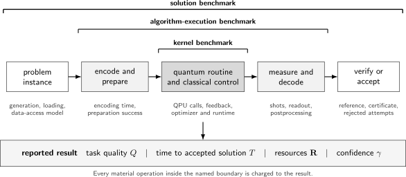
An algorithmic benchmark should name its boundary. A kernel benchmark isolates the central quantum computation. An execution benchmark includes preparation, hybrid control, and decoding. A solution benchmark includes the complete path from instance to accepted answer, together with quality, time, resources, and confidence.

The Algorithmic Benchmark Contract

For problem size $n$, define a benchmark by

$$\mathcal B_n = \left( \mathcal P_n, \Pi_n, \mathcal X, \mathcal A, \Lambda, \mathcal V_{\epsilon}, \mathcal S, \mathcal C \right).$$

The components are:

• $\mathcal P_n$: the problem family and output type;
• $\Pi_n$: the distribution or fixed corpus of instances;
• $\mathcal X$: the input encoding and access model;
• $\mathcal A$: the algorithm family;
• $\Lambda$: allowed variants, hyperparameters, and tuning budget;
• $\mathcal V_\epsilon$: the verifier or quality rule at tolerance $\epsilon$;
• $\mathcal S$: stopping, timeout, retry, and failure policy;
• $\mathcal C$: timing and resource boundary.

The implementation then maps an instance $I\sim\Pi_n$ and random seed $\omega$ to a reported output:

$$\widehat y = A_{\lambda,\omega}(I), \qquad \lambda\in\Lambda.$$

The benchmark score is conditional on the entire contract. A change from explicit matrix input to oracle access, from random initialization to a classically optimized warm start, or from one optimizer budget to another changes the algorithm being benchmarked.

Start from the Accepted Answer

For each instance $I$, define the set of acceptable outputs

$$\mathcal Y_\epsilon(I) = \left\{ y: L(I,y)\leq\epsilon \right\},$$

where $L$ is a task-specific loss. The success indicator for run $r$ is

$$Z_r = \mathbf 1 \left\{ \widehat y_r\in\mathcal Y_\epsilon(I_r) \right\}.$$

The conditional success probability is

$$p_{\mathrm s}(I) = \Pr \left[ \widehat y\in\mathcal Y_\epsilon(I) \mid I \right].$$

An ensemble benchmark may target the mean

$$\overline p_{\mathrm s}(n) = \mathbb E_{I\sim\Pi_n} \left[ p_{\mathrm s}(I) \right],$$

but a mean alone can hide a severe lower tail. Report instance quantiles or a failure fraction as well:

$$f_{\mathrm{fail}}(n) = \Pr_{I\sim\Pi_n} \left[ p_{\mathrm s}(I)<p_\star \right].$$

The output criterion should be frozen before test data are inspected. A success rule chosen after seeing the answers turns a benchmark into an uncontrolled selection procedure.

Success Is a Conditional Chain

An end-to-end run can fail during input validation, state preparation, algorithmic evolution, logical execution, measurement, decoding, or verification. Let these required events be $E_1,\ldots,E_K$. Then

$$\begin{aligned} p_{\mathrm{end}} &= \Pr(E_1\cap\cdots\cap E_K) \\ &= \Pr(E_1) \prod_{k=2}^{K} \Pr \left( E_k \mid E_1,\ldots,E_{k-1} \right). \end{aligned}$$

Multiplying independently estimated marginal success probabilities is valid only when the relevant independence assumptions hold. Conditional errors are often correlated: a poor state preparation can make the optimizer wander, drift can degrade several stages together, and postselection changes the distribution entering later analysis.

For approximation errors, a conservative additive budget often begins with a triangle or union-bound argument:

$$\epsilon_{\mathrm{tot}} \leq \epsilon_{\mathrm{enc}} + \epsilon_{\mathrm{alg}} + \epsilon_{\mathrm{synth}} + \epsilon_{\mathrm{noise}} + \epsilon_{\mathrm{sample}} + \epsilon_{\mathrm{decode}}.$$

This bound can be loose, but it prevents six individually “small” omissions from being silently treated as zero.

Cost per Accepted Solution

If independent runs have constant success probability $p_{\mathrm s}>0$ and each costs $C_{\mathrm{run}}$, the number of runs until the first success is geometric:

$$\Pr(R=r) = (1-p_{\mathrm s})^{r-1}p_{\mathrm s}.$$

Therefore

$$\mathbb E[R] = \frac{1}{p_{\mathrm s}},$$

and

$$\mathbb E[C_{\mathrm{solution}}] = \frac{C_{\mathrm{run}}}{p_{\mathrm s}}.$$

To obtain at least one success with confidence $\gamma$,

$$R_\gamma = \left\lceil \frac{\ln(1-\gamma)} {\ln(1-p_{\mathrm s})} \right\rceil.$$

If run durations vary, use the observed joint distribution of time and success rather than multiplying a mean time by a separately estimated retry count. Correlations matter when difficult instances are both slower and less likely to succeed.

Failed, timed-out, rejected, and postselected runs remain in the cost denominator. Reporting time only for the successful run estimates a conditional latency, not time to solution.

The End-to-End Cost Ledger

For a digital algorithm with $N_{\mathrm Q}$ quantum calls, one useful decomposition is

$$\begin{aligned} T_{\mathrm{end}} &= t_{\mathrm{ingest}} +t_{\mathrm{encode}} +t_{\mathrm{compile}} +t_{\mathrm{cal}} \\ &\quad+ \sum_{r=1}^{N_{\mathrm Q}} \left( t_{\mathrm{classical},r} +t_{\mathrm{comm},r} +t_{\mathrm{QPU},r} \right) \\ &\quad+ t_{\mathrm{decode}} +t_{\mathrm{verify}}. \end{aligned}$$

The resource record should accompany time:

$$\mathbf R = \left( N_{\mathrm Q}, N_{\mathrm{shots}}, N_{1q}, N_{2q}, D_{\mathrm{native}}, M_{\mathrm{peak}}, C_{\mathrm{class}}, E_{\mathrm{energy}} \right).$$

Add logical qubits, code cycles, non-Clifford resources, communication volume, queue time, human tuning, or monetary cost when they lie inside the claim. The goal is not to maximize the number of fields. It is to keep a material cost from disappearing because it occurs outside the QPU.

Adiabatic Quantum Computation supplies the fixed logical path, accepted-subspace decoder, schedule, gap/error certificate, and normalized AQC resource record for such a claim. This page retains the end-to-end time-to-accepted-answer ledger and fair comparator, including preparation, control, repetitions, readout, postprocessing, and validation.

Quantum Annealing owns the anneal-specific process record—schedule, declared regime, decoded success event, samples, gauges, embeddings, repeats, and per-run resources—that supplies inputs to this ledger. This page retains the complete end-to-end comparator, confidence, scaling, uncertainty, and advantage conclusion.

Input and Access Models

An algorithmic speedup theorem is conditional on how the input is supplied. Common access models include:

• an explicit classical array or sparse matrix;
• a circuit that prepares a quantum state;
• coherent query access to an oracle;
• a block encoding of an operator;
• local terms of a Hamiltonian;
• samples from a physical or statistical process;
• a stream whose preparation cost is outside the algorithm.

If the algorithm uses $N_{\mathrm q}$ oracle calls, the complete quantum cost has the schematic form

$$C_{\mathrm Q} = C_{\mathrm{encode}} + N_{\mathrm q}C_{\mathrm O} + C_{\mathrm{control}} + C_{\mathrm{read}} + C_{\mathrm{verify}}.$$

Treating $C_{\mathrm O}=1$ is appropriate for a query-complexity theorem. It is not appropriate for a hardware benchmark unless one physical oracle call really has the declared unit cost. The classical baseline must receive equivalent access to the same data.

Grover search as a diagnostic example

For one marked item among $N$, ideal Grover search uses approximately

$$N_{\mathrm q} \approx \frac{\pi}{4}\sqrt N$$

coherent predicate calls. A classical exhaustive search uses order $N$ predicate evaluations. If one coherent quantum predicate has cost $c_{\mathrm Q}$ and one classical evaluation costs $c_{\mathrm C}$, the leading work comparison is

$$C_{\mathrm Q} \approx \frac{\pi}{4}c_{\mathrm Q}\sqrt N, \qquad C_{\mathrm C} \approx \frac{1}{2}c_{\mathrm C}N.$$

Ignoring fixed costs, the quantum expression becomes smaller only beyond a constant-sensitive crossover:

$$\sqrt N \gtrsim \frac{\pi c_{\mathrm Q}} {2c_{\mathrm C}}.$$

The benchmark must also count superposition preparation, reflection, error correction, measurement, and candidate verification. Grover Search owns the algorithm and its optimal query bound; the calculation here illustrates why query count is not an end-to-end benchmark.

State Preparation and Useful Overlap

Many algorithms assume an input state

$$|\psi_0\rangle = \sum_j c_j|u_j\rangle.$$

If the desired eigenspace has projector $\Pi_\star$, its initial weight is

$$a_\star = \langle\psi_0| \Pi_\star |\psi_0\rangle.$$

An ideal phase-estimation run samples that sector with probability approximately $a_\star$, before finite-precision and implementation errors. The cost to prepare $|\psi_0\rangle$ and the retries associated with small $a_\star$ belong in the solution benchmark.

For a target confidence $\gamma$, an idealized repetition count is

$$R_\gamma = \left\lceil \frac{\ln(1-\gamma)} {\ln(1-a_\star p_{\mathrm{read}})} \right\rceil,$$

where $p_{\mathrm{read}}$ collects conditional algorithm and readout success. Supplying an exact eigenstate from a classical solver removes the hardest state-preparation problem and should be labeled as a conditional kernel test. Quantum Phase Estimation develops the precision law and overlap dependence.

Match the Metric to the Output Type

An algorithm’s output type determines its primary quality metric.

output type	primary benchmark quantity
decision	error probability, balanced accuracy, or risk under a declared prior
search	probability of a valid witness and cost per verified witness
estimation	bias, variance, mean-squared error, and confidence coverage
sampling	task-relevant distribution distance or validated observables
optimization	feasible objective quality, optimality gap, or approximation ratio
simulation	error in declared observables, times, and initial states
learned model	held-out loss, calibration, sample efficiency, and training cost

A gate fidelity or overlap may be a useful diagnostic for any row, but it does not replace the output-level metric.

Decision Problems

For a binary decision with truth $Y\in\{0,1\}$ and prediction $\widehat Y$, the risk under prior $\pi$ is

$$R_\pi = \pi\, \Pr(\widehat Y=0\mid Y=1) + (1-\pi)\, \Pr(\widehat Y=1\mid Y=0).$$

If the test corpus is class imbalanced, raw accuracy can be misleading. Balanced accuracy is

$$A_{\mathrm{bal}} = \frac{1}{2} \left[ \Pr(\widehat Y=1\mid Y=1) + \Pr(\widehat Y=0\mid Y=0) \right].$$

Benchmark both yes- and no-instances and preserve the intended prior. A one-sided corpus can reward an implementation that always emits the same answer.

For bounded-error algorithms, state whether repetition and majority voting are part of the implementation. Their quantum calls and classical vote time belong in the cost.

Estimation Problems

For an estimator $\widehat\theta$ of $\theta$, the mean-squared error is

$$\operatorname{MSE} \left( \widehat\theta \right) = \mathbb E \left[ (\widehat\theta-\theta)^2 \right].$$

It decomposes as

$$\operatorname{MSE} = \operatorname{Bias}^2 + \operatorname{Var}.$$

Report both terms when coherent bias, mitigation bias, finite precision, or optimizer bias may be material. An algorithm can have small shot variance and a large systematic error.

The benchmark should vary the requested tolerance and confidence:

$$C(\epsilon,\gamma) = \text{cost to achieve } \Pr \left( |\widehat\theta-\theta| \leq\epsilon \right) \geq\gamma.$$

This function is more informative than one error value at one arbitrary shot count. Confidence intervals should be checked for coverage on instances with known answers, not merely reported.

Search and Optimization Problems

For a maximization problem with feasible set $\mathcal F(I)$ and objective $f_I(x)$, every reported sample should first pass feasibility:

$$x\in\mathcal F(I).$$

An optimality gap is

$$\Delta_f(x) = f_I^\star-f_I(x),$$

where $f_I^\star$ is known exactly or bounded by a trusted reference. An approximation ratio may be useful when signs and normalization are well-defined:

$$\rho(x) = \frac{f_I(x)}{f_I^\star}.$$

For objectives that may be negative, shifted, or zero, this ratio can be unstable or reverse ordering. A baseline-normalized score for maximization is

$$s(x) = \frac{ f_I(x)-f_{\mathrm{base}}(I) }{ f_{\mathrm{ref}}(I)-f_{\mathrm{base}}(I) }.$$

The baseline and reference are part of the metric; changing either changes the score. Publish raw objective values and feasibility alongside any normalization.

For a target quality $f_\star(I)$, define

$$p_\star(I) = \Pr \left[ x\in\mathcal F(I), \quad f_I(x)\geq f_\star(I) \right].$$

Time to target then includes optimization, sampling, and retries. “Best of $K$ samples” must report $K$ because increasing $K$ improves the expected best objective even if the sampler is unchanged.

Sampling Problems

For target distribution $p$ and measured distribution $q$, total-variation distance is

$$D_{\mathrm{TV}}(p,q) = \frac{1}{2} \sum_x |p(x)-q(x)|.$$

This is operationally meaningful, but estimating it for a large unstructured outcome space can require prohibitive samples and a classically available reference. A scalable algorithmic benchmark may instead validate:

• selected marginals or correlators;
• conserved quantities and symmetries;
• efficiently computable witnesses;
• held-out task statistics;
• smaller exact instances and overlap regions;
• cross-platform or interactive checks.

Those tests certify only their declared properties. Matching a few observables does not imply small total-variation distance. Cross-Entropy Benchmarking explains the analogous gap for random-circuit scores.

Sample generation rate should count discarded and correlated outputs. If successive samples have autocorrelation time $\tau_{\mathrm{int}}$, a rough effective sample size is

$$N_{\mathrm{eff}} \approx \frac{N} {2\tau_{\mathrm{int}}}.$$

Quoting raw sample rate without independence diagnostics can overstate statistical throughput.

Simulation Algorithms

For a quantum simulation task, define the model, initial state, observable set $\mathcal O$, and time grid $\mathcal T$. One aggregate error is

$$E_{\mathrm{sim}} = \sum_{O\in\mathcal O} w_O \sum_{t\in\mathcal T} w_t \left| \widehat{\langle O(t)\rangle} - \langle O(t)\rangle_{\mathrm{ref}} \right|^2.$$

The weights encode scientific priorities and must be published. A useful record also separates:

• model-discretization or truncation error;
• state-preparation error;
• product-formula or algorithmic approximation;
• synthesis and hardware error;
• finite-shot uncertainty;
• reference-solver uncertainty.

One well-matched observable at one time does not validate a trajectory. What Is Quantum Simulation? owns the larger mapping, validation, and scientific-use workflow.

Hybrid Quantum–Classical Algorithms

Variational Quantum Algorithms owns the parameterized-circuit, estimator, gradient, trainability, and optimization machinery. Quantum Machine Learning owns the learning task, data, split, and generalization semantics; this page retains the full comparator, statistics, and cost protocol. At the benchmark boundary, a variational or adaptive algorithm generates a stochastic trajectory:

$$\theta_{r+1} = \mathcal O \left( \theta_r, \widehat g_r, \eta_r \right),$$

where $\mathcal O$ is the classical update rule, $\widehat g_r$ is estimated from quantum data, and $\eta_r$ collects optimizer randomness. The benchmark output depends on:

• initialization;
• ansatz and parameterization;
• optimizer and hyperparameters;
• measurement grouping and shot allocation;
• stopping and restart rules;
• mitigation and calibration;
• classical numerical precision;
• communication latency.

The complete call count is

$$N_{\mathrm Q} = \sum_{r=1}^{R} \sum_{g=1}^{G_r} N_{\mathrm{circuits}}(r,g),$$

where $G_r$ may index measurement groups, shifted parameters, or adaptive queries. The total shots are

$$N_{\mathrm{shots}} = \sum_{r,g,c} S_{r,g,c}.$$

Reporting only the final circuit depth discards the dominant work when hundreds or thousands of circuits were used to discover its parameters.

Frozen-parameter and trained modes

Two benchmark modes answer different questions:

• frozen-parameter mode supplies parameters in advance and evaluates the quantum circuit and readout path;
• trained mode begins from the declared initialization and includes the full optimization process.

The first isolates execution quality. The second evaluates the algorithm. Calling the first “end-to-end VQE” or “end-to-end QAOA” is inaccurate unless parameter discovery is genuinely outside the intended task.

Variational energy example

For Hamiltonian

$$H = \sum_{\alpha=1}^{M} h_\alpha P_\alpha,$$

the variational energy is

$$E(\theta) = \sum_{\alpha=1}^{M} h_\alpha \langle P_\alpha\rangle_\theta.$$

An algorithmic benchmark should report final energy error,

$$\Delta E = E(\widehat\theta)-E_0,$$

together with total quantum calls, shots, optimizer iterations, wall time, restart distribution, and any classical preprocessing used to choose the ansatz or warm start. A low energy does not by itself imply high state fidelity when low-lying levels are dense.

Algorithm Variants and Tuning Budgets

An algorithm name usually denotes a family:

$$A_\lambda, \qquad \lambda\in\Lambda.$$

The configuration $\lambda$ may include:

• ansatz depth or product-formula order;
• phase-register precision;
• synthesis tolerance;
• measurement allocation;
• optimizer and learning rate;
• mitigation strength;
• decoder or postprocessing method;
• compiler and placement seed.

There are two defensible policies.

Fixed-configuration comparison

Choose $\lambda$ before evaluation and apply the same mathematical configuration to every system. This isolates execution differences but may favor one architecture.

Equal-budget best-stack comparison

Give every system the same declared tuning budget $B$ and report the best held-out configuration:

$$\widehat\lambda = \operatorname*{arg\,min}_{\lambda\in\Lambda_B} \widehat L_{\mathrm{validation}}(\lambda).$$

Then evaluate $\widehat\lambda$ on untouched test instances. This measures a delivered workflow, including compiler and algorithm selection.

Searching many configurations and reporting the best test score overfits the benchmark. The number of attempted configurations, tuning time, and validation procedure are resources.

Error Mitigation and Postselection

Mitigation can improve output quality while increasing variance, shots, circuit count, classical work, and latency. Report a quality–cost pair:

$$\left( Q_{\mathrm{raw}}, C_{\mathrm{raw}} \right), \qquad \left( Q_{\mathrm{mit}}, C_{\mathrm{mit}} \right).$$

For postselection event $A$, the acceptance rate is

$$a = \Pr(A).$$

If $N_{\mathrm{keep}}$ accepted samples are needed, the expected raw count is

$$\mathbb E[N_{\mathrm{raw}}] \approx \frac{N_{\mathrm{keep}}}{a}.$$

The selected output distribution is

$$q(x\mid A) = \frac{q(x,A)}{a}.$$

It answers a conditional task. The benchmark must state whether rejection is allowed operationally and include rejected runs in time and resource totals. Noise in Quantum Information owns the device-facing noise-model context. Error Mitigation Overview owns mitigation-estimator licenses, covariance, acceptance, calibration, stacking, and method-level resource accounting; this page retains the end-to-end algorithm benchmark and cost-to-accepted-answer comparison.

Limits of Error Mitigation owns the theorem hypotheses, mitigation-specific scaling bounds, and finite stress tests that can disqualify a mitigation claim; this page retains the complete task, comparator, and time-to-accepted-answer benchmark.

Reference Answers and Verification

An algorithmic benchmark needs a trustworthy way to score outputs. A useful verification ladder is:

1. analytic answers and identities;
2. exact classical computation for small instances;
3. independently implemented numerical methods in an overlap regime;
4. rigorous upper and lower bounds;
5. efficiently checkable witnesses or certificates;
6. conserved quantities and metamorphic relations;
7. cross-device or interactive verification;
8. domain validation against experiment or trusted data.

Reference uncertainty belongs in the loss. If

$$|\theta_{\mathrm{ref}}-\theta| \leq \epsilon_{\mathrm{ref}}$$

and the measured discrepancy is

$$|\widehat\theta-\theta_{\mathrm{ref}}| \leq \epsilon_{\mathrm{meas}},$$

then a conservative bound is

$$|\widehat\theta-\theta| \leq \epsilon_{\mathrm{meas}} + \epsilon_{\mathrm{ref}}.$$

Do not label a simulator “exact” merely because it is classical. Truncation, floating-point, convergence, and implementation errors require validation too.

Instance Families and Scaling Variables

Problem size $n$ rarely determines difficulty by itself. Define an instance feature vector

$$\phi(I) = \left( n, \kappa, s, \Delta, \chi, \ldots \right),$$

where the entries might include condition number $\kappa$, sparsity $s$, spectral gap $\Delta$, graph density, entanglement structure $\chi$, precision, or another task-relevant parameter.

Benchmark at:

• fixed features while varying $n$;
• fixed $n$ while varying hardness features;
• realistic joint distributions;
• adversarial and edge-case strata;
• analytically soluble and independently verifiable overlap regions.

An algorithm whose theorem scales as $\operatorname{poly}(\kappa)$ should not be benchmarked only on matrices with $\kappa=1$ and then advertised as a general linear solver.

Measuring Scaling

Suppose quantum and classical solution costs are modeled as

$$C_{\mathrm Q}(n,\epsilon) = A_{\mathrm Q} f_{\mathrm Q}(n,\epsilon),$$

and

$$C_{\mathrm C}(n,\epsilon) = A_{\mathrm C} f_{\mathrm C}(n,\epsilon).$$

A crossover solves

$$C_{\mathrm Q}(n_\times,\epsilon) = C_{\mathrm C}(n_\times,\epsilon).$$

This equation is useful only if:

• both sides solve the same task at the same tolerance and confidence;
• all material constants and overheads are included;
• the tested sizes constrain the proposed scaling functions;
• the classical implementation is competitive;
• uncertainty in fitted parameters is propagated to $n_\times$.

Three small points do not establish an asymptotic exponent. Report raw data, residuals, alternative plausible models, and prediction intervals. Avoid discarding setup costs merely because they are asymptotically lower order; they can dominate every reachable instance.

Strong and weak scaling

Two distinct experiments are useful:

• strong scaling: hold the instance fixed and vary available hardware or parallel resources;
• weak or problem scaling: increase the instance while changing resources according to a declared rule.

Mixing them can make runtime appear flat because both problem size and machine capacity changed.

Classical Baselines without Overclaiming

Classical Information Review supplies the source–channel–code–decoder, access, error, and cost ledger for a fair baseline. This page owns the executable task contract, tuning policy, scaling study, and cost-to-accepted-solution evidence.

An algorithm benchmark should usually include:

• a transparent simple baseline;
• a strong domain-specific baseline;
• the best available implementation the study can reasonably access;
• ablations showing which quantum and classical components matter.

Match:

• input representation and preprocessing;
• output tolerance and confidence;
• hardware and parallelism accounting;
• warm starts and tuning budgets;
• timeout and failure treatment;
• inclusion of verification.

The result may still be valuable when the classical method wins. It can identify bottlenecks, validate the implementation, and establish the regime that future systems must improve.

Be precise about evidence categories:

$$\text{algorithm theorem} \neq \text{resource estimate} \neq \text{hardware execution} \neq \text{advantage demonstration}.$$

Quantum Complexity Classes owns asymptotic computational classes, while Claims, Hype, and Evidence Standards owns public claim calibration.

Fault-Tolerant Algorithmic Benchmarks

For an error-corrected execution, the logical algorithm is only the beginning. The benchmark record may need:

• logical input and output contract;
• code family and distance schedule;
• non-Clifford state factories;
• routing and lattice-surgery schedule;
• decoder latency and classical throughput;
• logical failure budget by subroutine;
• verification and restart policy;
• physical qubits, cycles, energy, and elapsed time.

If subroutine $j$ has failure probability $p_j$, a union bound gives

$$p_{\mathrm{fail}} \leq \sum_j p_j.$$

Assigning every subroutine the same $p_j$ can be wasteful. A mature design allocates the failure budget jointly with factory, code-distance, and runtime optimization.

Predicted fault-tolerant performance is a resource estimate, not a measured benchmark. An experimental algorithmic benchmark becomes possible when the encoded system actually executes the declared task and its logical failures, rate, decoding, and overhead are observed.

Statistical Hierarchy

Algorithmic data are commonly nested:

$$\text{day} \supset \text{instance} \supset \text{initialization} \supset \text{optimizer seed} \supset \text{circuit} \supset \text{shot}.$$

The uncertainty target determines the resampling unit. Shot resampling quantifies measurement noise conditional on one circuit. It does not generalize to new instances or optimizer seeds.

For quality $Q_{i,r}$ on instance $i$ and run $r$, an ensemble mean is

$$\widehat\mu_Q = \frac{1}{N_I} \sum_{i=1}^{N_I} \left( \frac{1}{R_i} \sum_{r=1}^{R_i} Q_{i,r} \right).$$

Equal instance weighting differs from pooling every run when $R_i$ varies. Choose the estimand deliberately.

Report:

• between-instance variation;
• within-instance stochastic variation;
• time-block drift;
• uncertainty in reference answers;
• dependence between quality and time;
• multiplicity from trying sizes, variants, or subsets.

A hierarchical bootstrap or model can combine these levels, but its structure must match the actual sampling process.

Reproducible Execution Record

Preserve:

• task and instance generator with checksums;
• train, validation, and test partitions;
• input encodings, oracles, state-preparation circuits, and data-loading code;
• algorithm variant, hyperparameters, random seeds, and stopping rule;
• source, lowered, native, and scheduled programs;
• hardware, firmware, calibration, compiler, and runtime versions;
• all quantum counts and intermediate classical states;
• optimizer trajectory and restart history;
• raw, mitigated, and postselected outputs;
• timing events with clock source and boundary;
• failed, rejected, cancelled, and timed-out runs;
• reference-solver code, tolerances, and uncertainty;
• analysis environment and exact score computation.

Reproducible Notebooks develops the executable evidence bundle, while Circuit Intermediate Representations owns the versioned program artifacts.

A Defensible Workflow

1. Define the problem. State input, output, tolerance, confidence, and operational success.
2. Choose the boundary. Name kernel, execution, or solution scope.
3. Freeze instances. Specify the population, features, partitions, seeds, and held-out policy.
4. Freeze access. Document data loading, oracle, state preparation, and what each baseline receives.
5. Select metrics. Use task-level quality plus timing and a resource vector.
6. Budget variants. Equalize or declare algorithm, compiler, mitigation, and tuning freedom.
7. Validate references. Use analytic cases, independent implementations, and overlap regimes.
8. Run hierarchical repetitions. Sample instances, seeds, time blocks, circuits, and shots at the levels relevant to the claim.
9. Publish trajectories and failures. Do not retain only the best final point.
10. Analyze scaling cautiously. Include constants, alternatives, and uncertainty before projecting a crossover.
11. Compare matched baselines. Equalize task, accuracy, access, and resource boundaries.
12. Scope the conclusion. State exactly what was executed, estimated, or extrapolated.

Minimum Reporting Record

• problem statement and benchmark boundary;
• instance distribution, feature strata, and tested sizes;
• input and oracle access model;
• accepted-output rule, tolerance, and confidence;
• algorithm version and every adaptive choice;
• initialization, optimizer, restart, stopping, and timeout policy;
• circuit, shot, and quantum-call totals;
• native counts, schedule, mapping, and compiler record;
• raw and mitigated quality;
• postselection acceptance and all failed runs;
• complete timing boundary and event timestamps;
• classical compute, memory, and parallelism;
• reference method and uncertainty;
• per-instance and per-run results;
• hierarchical uncertainty and multiplicity treatment;
• scaling model, alternatives, and prediction interval;
• dated hardware, software, and calibration provenance.

Common Mistakes

Benchmarking the circuit instead of the algorithm

Ideal parameters, exact input states, or simulator-selected outputs can remove the hard part of the task. Label the result as a kernel test.

Counting oracle calls as wall-clock time

Query complexity is conditional on an access model. Implement and count the oracle, or keep the claim explicitly query theoretic.

Ignoring state-preparation overlap

An algorithm can have excellent conditional accuracy and negligible probability of entering the useful subspace.

Reporting only successful runs

Retries, timeouts, rejected samples, and optimizer failures determine cost to solution.

Freezing parameters without saying so

A fixed variational circuit does not measure the training loop.

Comparing unequal accuracy

A faster but less accurate output is not a speed result at matched task quality. Publish a quality–cost frontier.

Using only easy instances

One problem-size integer does not characterize condition number, density, gap, or structure. Stratify the instance family.

Fitting an exponent to a few points

Small-instance trends can reflect fixed overhead, compiler thresholds, or classical simulation artifacts rather than asymptotic scaling.

Treating mitigation as free

Count noise-scaled circuits, rejected samples, extra shots, classical postprocessing, and induced bias.

Calling a benchmark an advantage demonstration

Algorithm quality is necessary evidence, but advantage requires a separate matched classical-frontier and verification case.

Research Status

End-to-end task definitions, matched accuracy, complete timing boundaries, instance distributions, and reproducible statistical reporting are established principles of scientific benchmarking. Application-oriented quantum benchmark suites and full-stack circuit methods now provide practical frameworks for applying them.

Several issues remain active: scalable verification after exact simulation fails; benchmark governance and hidden instances; fair accounting for tuning, mitigation, and cloud services; representative hybrid workloads; logical algorithm benchmarks; energy and cost measurement; and robust extrapolation to useful scales. Recent studies increasingly report complete quantum– classical loops and strong baselines, but terminology is not yet standardized.

The durable rule is that an algorithm is benchmarked only when the benchmark preserves the task it is meant to solve.

Further Connections

• Quantum Volume and Application Benchmarks owns suite construction, width–depth maps, and cross-platform implementation policy.
• Digital Quantum Simulation gives a complete application workflow whose encoding, approximation, compilation, execution, sampling, and validation costs must remain inside a task-preserving benchmark.
• Why Benchmarking Is Hard supplies the general estimand, drift, selection, verification, and reporting contract.
• Reporting Standards specifies the hardware, executable, optimizer, acquisition, mitigation, postselection, uncertainty, resource, code, and data record for an algorithm result.
• Verification of Quantum Advantage adds the correctness, hardness, dated classical-frontier, adversarial, and reproduction evidence required before algorithm performance becomes an advantage claim.
• Algorithmic Primitives distinguishes query, gate, state-preparation, output, and fault-tolerant resources.
• Grover Search gives the exact success law and optimal coherent-query bound.
• Quantum Phase Estimation develops overlap, precision, evolution-time, and readout costs.
• VQE applies the end-to-end benchmark contract to Hamiltonian construction, adaptive energy search, independent validation, and matched classical baselines.
• Quantum Chemistry Case Studies applies that contract to experimental molecular runs, active-space model ladders, and conditional fault-tolerant projections.
• Shor Algorithm provides a complete probabilistic pipeline with efficient classical verification and model-dependent fault-tolerant estimates.
• Quantum Complexity Classes separates asymptotic computational statements from practical performance.
• What Is Quantum Simulation? defines model mapping, observable validation, and scientific baselines.
• Quantum Software Stack identifies every classical and quantum layer inside an execution.
• Resource Estimation Tools develops conditional logical and physical predictions.
• Noise in Quantum Information supplies the noise-model context for mitigation estimators, bias, variance, and sampling overhead.
• Claims, Hype, and Evidence Standards separates theorem, estimate, benchmark, application, and advantage claims.

References

1. T. Proctor, K. Young, A. D. Baczewski, and R. Blume-Kohout, “Benchmarking quantum computers,” Nature Reviews Physics 7, 105–118 (2025), doi:10.1038/s42254-024-00796-z.
2. T. Lubinski et al., “Application-oriented performance benchmarks for quantum computing,” IEEE Transactions on Quantum Engineering 4, 3100316 (2023), doi:10.1109/TQE.2023.3253761.
3. T. Lubinski et al., “Quantum algorithm exploration using application-oriented performance benchmarks,” arXiv:2402.08985 (2024), arXiv:2402.08985. This remains a preprint and evolving extension of the QED-C methodology.
4. J. R. Finžgar, P. Ross, L. Hölscher, J. Klepsch, and A. Luckow, “QUARK: A framework for quantum computing application benchmarking,” in 2022 IEEE International Conference on Quantum Computing and Engineering, 226–237 (2022), doi:10.1109/QCE53715.2022.00042.
5. J. Hines and T. Proctor, “Scalable full-stack benchmarks for quantum computers,” IEEE Transactions on Quantum Engineering 5, 1–12 (2024), doi:10.1109/TQE.2024.3404502.
6. T. Hoefler and R. Belli, “Scientific benchmarking of parallel computing systems: twelve ways to tell the masses when reporting performance results,” in SC ’15: Proceedings of the International Conference for High Performance Computing, Networking, Storage and Analysis, 73:1–73:12 (2015), doi:10.1145/2807591.2807644.
7. K. Bharti et al., “Noisy intermediate-scale quantum algorithms,” Reviews of Modern Physics 94, 015004 (2022), doi:10.1103/RevModPhys.94.015004.
8. M. Cerezo et al., “Variational quantum algorithms,” Nature Reviews Physics 3, 625–644 (2021), doi:10.1038/s42254-021-00348-9.
9. J. Tilly et al., “The variational quantum eigensolver: a review of methods and best practices,” Physics Reports 986, 1–128 (2022), doi:10.1016/j.physrep.2022.08.003.
10. R. Babbush et al., “Focus beyond quadratic speedups for error-corrected quantum advantage,” PRX Quantum 2, 010103 (2021), doi:10.1103/PRXQuantum.2.010103.
11. A. M. Dalzell et al., “End-to-end resource analysis for quantum interior-point methods and portfolio optimization,” PRX Quantum 4, 040325 (2023), doi:10.1103/PRXQuantum.4.040325.
12. L. K. Grover, “A fast quantum mechanical algorithm for database search,” in Proceedings of the 28th Annual ACM Symposium on Theory of Computing, 212–219 (1996), doi:10.1145/237814.237866.
13. P. W. Shor, “Algorithms for quantum computation: discrete logarithms and factoring,” in Proceedings of the 35th Annual Symposium on Foundations of Computer Science, 124–134 (1994), doi:10.1109/SFCS.1994.365700.
14. A. Peruzzo et al., “A variational eigenvalue solver on a photonic quantum processor,” Nature Communications 5, 4213 (2014), doi:10.1038/ncomms5213.
15. Z. Cai et al., “Quantum error mitigation,” Reviews of Modern Physics 95, 045005 (2023), doi:10.1103/RevModPhys.95.045005.
16. J. Tuziemski, J. Pawłowski, P. Tarasiuk, Ł. Pawela, and B. Gardas, “Limits of quantum run-time advantage,” Physical Review Applied 25, 044084 (2026), doi:10.1103/gpsf-pn1x.

Exercises

1. Distinguish benchmark boundaries

A study prepares a VQE circuit at parameters obtained by exact diagonalization, measures its energy, and compares the result with the exact ground-state energy. Is this a kernel, execution, or solution benchmark? What must be added to reach the next two boundaries?

Solution

It is a kernel benchmark: it tests circuit preparation, measurement, and energy estimation at externally supplied parameters. An execution benchmark would include parameter initialization, optimizer, shot allocation, iterations, stopping rule, and restarts. A solution benchmark would also include constructing the Hamiltonian from the declared instance, ingesting the input, defining the accepted energy tolerance, verifying the final result, handling failures, and counting all quantum and classical time and resources.

2. Include state overlap in cost

Phase estimation has conditional readout success $p_{\mathrm{read}}=0.8$ once the target eigenspace is occupied. The prepared state has target weight $a_\star=0.05$. Each run takes $2$ s. Estimate the number of independent runs and time needed for at least $95\%$ chance of one accepted result.

Solution

The per-run success probability is

$$p_{\mathrm s} = a_\star p_{\mathrm{read}} = 0.04.$$

Thus

$$R_{0.95} = \left\lceil \frac{\ln(0.05)} {\ln(0.96)} \right\rceil = 74.$$

The idealized time is

$$T_{0.95} = 74(2\ \mathrm s) = 148\ \mathrm s.$$

This excludes setup and assumes stationary independent runs.

3. Expose a hidden oracle cost

A quantum search uses $(\pi/4)\sqrt N$ oracle calls, each taking $10^4$ times as long as one classical predicate evaluation. A classical search uses approximately $N/2$ evaluations. Ignoring fixed costs, estimate the crossover scale.

Solution

Set

$$\frac{\pi}{4} 10^4\sqrt N \approx \frac{N}{2}.$$

Then

$$\sqrt N \approx \frac{\pi}{2}10^4,$$

so

$$N \approx \frac{\pi^2}{4}10^8 \approx 2.47\times10^8.$$

The query advantage does not translate into lower work until very large $N$ under this cost ratio, even before state preparation, error correction, and verification are counted.

4. Compute cost per accepted result

An optimizer run succeeds with probability $0.25$. Successful runs average $40$ s, while failed runs average $20$ s. Runs are independent. What is the expected time to the first success?

Solution

The expected number of failures before the first success is

$$\frac{1-p_{\mathrm s}}{p_{\mathrm s}} = \frac{0.75}{0.25} = 3.$$

Therefore

$$\mathbb E[T] = 3(20\ \mathrm s) + 40\ \mathrm s = 100\ \mathrm s.$$

Using an unconditional mean run time divided by $p_{\mathrm s}$ gives the same answer only if the mean is formed with the correct success–time mixture.

5. Repair an optimization score

A maximization task can have negative optimum. Explain why $\rho=f(x)/f^\star$ may be misleading and propose a safer reported record.

Solution

When $f^\star<0$, a worse solution can produce a ratio larger than one or reverse ordering; when $f^\star$ is near zero, the ratio is unstable. Report feasibility, raw objective $f(x)$, and gap $f^\star-f(x)$ when a trusted optimum or bound exists. A baseline-normalized score can be added if its baseline and reference are explicit, but raw values and uncertainty should remain visible.

6. Count postselection overhead

A mitigation protocol accepts $12\%$ of raw shots. The final analysis needs $6\,000$ accepted samples. Estimate the expected raw shots. What additional evidence is needed before interpreting the selected result?

Solution

The expected raw count is

$$\mathbb E[N_{\mathrm{raw}}] \approx \frac{6000}{0.12} = 50\,000.$$

The benchmark must report the acceptance event, raw and selected distributions, uncertainty in the acceptance rate, all time and cost for rejected shots, and whether conditioning preserves the intended task rather than changing it.

7. Design an estimation benchmark

Give a minimal benchmark for an energy estimator that distinguishes bias, variance, and confidence calibration.

Solution

Choose held-out Hamiltonians with trusted energies and a range of sizes, spectral gaps, and term structures. For each, repeat the full algorithm across independent seeds and time blocks at several shot budgets. Report signed error, bias, variance, MSE, interval width, and empirical coverage at the declared confidence. Include state preparation, grouping, mitigation, classical processing, failed runs, and reference uncertainty. Plot cost versus tolerance and confidence rather than one error at one shot count.

8. Audit a scaling claim

A paper measures quantum runtimes at $n=6,8,10$ and classical runtimes at $n=50,100,200$, fits separate exponentials, and predicts a crossover at $n=30$. List the main problems.

Solution

The quantum and classical fits use disjoint regimes; three quantum points do not constrain an asymptotic model; the predicted crossover lies outside the quantum data; instance distributions and accuracy may differ; fixed preparation, communication, and verification costs may be omitted; and model and parameter uncertainty may not be propagated. A repair uses matched instances or controlled feature distributions, identical output tolerance, overlapping sizes, strong implementations, complete timing, alternative models, residual checks, and a prediction interval. If no overlap is feasible, the result should be labeled a conditional projection rather than an observed crossover.