Quantum Chemistry Case Studies

Short Definition

A quantum chemistry case study follows one scientific question through molecular modeling, finite-basis Hamiltonian construction, quantum encoding, algorithm execution or resource estimation, classical comparison, and claim validation. The important output is not merely an energy number. It is an auditable statement of what was calculated, which approximations were made, what the quantum processor actually did, and what the result establishes.

This page compares representative experiments and fault-tolerant projections. The cases were selected because they expose recurring issues:

• hydrogen demonstrates complete small-instance pipelines;
• lithium hydride and beryllium hydride expose hardware-aware VQE tradeoffs;
• water separates executed circuits from the larger proposed ansatz and shows the first logical-encoding demonstrations;
• nitrogen tests bond breaking, active subspaces, and multireference behavior;
• FeMoco, ruthenium catalysis, and cytochrome P450 expose the assumptions inside fault-tolerant resource estimates.

VQE owns the variational algorithm and its energy-specific error budget. Quantum Phase Estimation owns phase resolution and coherent-time costs. Electronic Structure Overview owns basis sets, correlation methods, and chemistry-model approximations. This page owns the comparison of complete case-study claims. Simulation of Quantum Chemistry owns the general molecular-model, encoding, solver, observable, resource, and validation workflow used to interpret those cases.

How to Read a Chemistry Demonstration

For every reported molecular calculation, ask six questions.

1. Scientific target: Is the goal an absolute energy, energy difference, potential-energy curve, equilibrium geometry, excitation, spin gap, reaction barrier, or response property?
2. Encoded model: Which geometry, basis, pseudopotential, frozen orbitals, active space, relativistic terms, charge, spin, and symmetry sector define the Hamiltonian?
3. Quantum task: Did hardware optimize a state, measure a state whose parameters came from classical simulation, execute phase estimation, or only run a kernel from a proposed workflow?
4. Evidence: Is the result a noiseless numerical study, a physical-device experiment, an error-detecting logical experiment, or a conditional fault-tolerant estimate?
5. Baseline: Was the same finite Hamiltonian compared with exact diagonalization, a selected classical approximation, or the strongest tractable classical method?
6. Claim: Does the result establish circuit control, algorithmic accuracy for a toy model, chemical usefulness, favorable projected resources, or computational advantage?

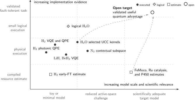
Quantum chemistry evidence currently occupies two complementary regions. Physical experiments provide execution evidence for small or heavily reduced models. Chemically ambitious targets occupy the resource-estimate region. Movement toward the open upper-right target requires both a scientifically adequate model and a validated end-to-end quantum computation; progress along only one axis is not equivalent to practical advantage.

Evidence labels

The following labels are deliberately narrower than “quantum simulation”:

Label	What happened	What it can support
Compiled demonstration	A small, instance-specific circuit was executed	Control and readout of that circuit
Algorithmic hardware run	A scalable algorithmic structure was executed on a tractable model	End-to-end behavior at that scale
Quantum kernel run	Hardware evaluated selected states, terms, or subroutines while substantial work remained classical	Performance of the executed kernel
Logical demonstration	Encoded states or logical operations were used, often with detection or postselection	Behavior of that code-and-circuit instance
Resource estimate	An algorithm was compiled through a declared fault-tolerant model	Conditional requirements under those assumptions
Advantage experiment	A useful accepted answer beats the dated classical frontier under matched resources	A scoped computational-advantage claim

The same paper can legitimately carry more than one label. The label should attach to a specific claim, not to an entire research program.

The Layered Error Ledger

Let $E_{\mathrm{phys}}$ denote the exact value for the intended physical model and let $E_{\mathrm{enc}}$ be the exact ground energy of the finite encoded Hamiltonian. A diagnostic decomposition is

$$\begin{aligned} \widehat E-E_{\mathrm{phys}} ={}& \left( \widehat E-E_{\mathrm{impl}} \right) + \left( E_{\mathrm{impl}}-E_{\Theta} \right) \\ &+ \left( E_{\Theta}-E_{\mathrm{enc}} \right) + \left( E_{\mathrm{enc}}-E_{\mathrm{phys}} \right). \end{aligned}$$

Here:

• $\widehat E-E_{\mathrm{impl}}$ contains finite sampling, readout, drift, and mitigation effects;
• $E_{\mathrm{impl}}-E_\Theta$ contains implementation and optimization effects relative to the intended trial family;
• $E_\Theta-E_{\mathrm{enc}}$ is representation error within the encoded problem;
• $E_{\mathrm{enc}}-E_{\mathrm{phys}}$ is chemistry-model error.

These terms are not always independently observable, and nonlinear postprocessing can make a literal additive attribution inappropriate. The ledger is still useful because it prevents a small first term from being reported as a small total error.

For a potential-energy curve, write the encoded-model deviation as

$$\Delta(R) = E_{\mathrm{method}}(R) - E_{\mathrm{reference}}(R).$$

The nonparallelity error

$$\operatorname{NPE} = \max_R\Delta(R) - \min_R\Delta(R)$$

measures distortion of the curve after removing a constant offset. It can be more informative than the best error at one geometry. Equilibrium bond lengths, dissociation energies, barriers, and state crossings require their own derived uncertainty analysis.

Case Study: Hydrogen as a Pipeline Test

Molecular hydrogen is the smallest nontrivial electronic-structure benchmark. In a minimal spatial basis with two orbitals, there are four spin orbitals. Second-quantized encodings therefore begin with four qubits, while fixed particle number, spin parity, and other symmetries can reduce the executable problem further.

In a sector with $N_\alpha$ spin-up and $N_\beta$ spin-down electrons among $M$ spatial orbitals, the determinant count is

$$D = \binom{M}{N_\alpha} \binom{M}{N_\beta}.$$

For minimal-basis hydrogen this space is tiny enough to diagonalize exactly on a classical computer. That makes it an excellent validation target and an inappropriate target for a computational-advantage claim.

Photonic phase estimation in 2010

Lanyon and collaborators used a photonic processor to calculate the minimal-basis hydrogen spectrum with a phase-estimation architecture. The experiment reported high numerical phase precision and demonstrated iterative ideas relevant to molecular eigenvalue estimation.

The correct interpretation is narrower than “large-scale chemistry solved by phase estimation.” The molecular Hamiltonian was extremely small, and instance-specific compilation moved substantial work outside the executed circuit. The result validated optical control, phase readout, and a small chemistry mapping. It did not validate scalable Hamiltonian simulation, ground-state preparation, or the fault-tolerant cost of obtaining the same precision for a classically difficult molecule.

Superconducting VQE and phase estimation in 2016

O’Malley and collaborators calculated the hydrogen dissociation curve on superconducting hardware with both unitary-coupled-cluster VQE and a Trotterized phase-estimation route. Unlike earlier demonstrations that relied on exponentially costly precompilation, the VQE circuit retained a scalable algorithmic structure. The experiment reached the conventional $1.6\,\mathrm{m}E_{\mathrm h}$ algorithmic-accuracy threshold for its encoded problem and illustrated that the short VQE circuit was more tolerant of some device errors than the deeper phase-estimation circuit.

Three qualifications remain:

• the minimal-basis Hamiltonian was classically trivial;
• agreement with exact diagonalization tested algorithmic error, not complete basis or experimental chemical accuracy;
• the favorable depth comparison did not include the asymptotic precision advantage available to fault-tolerant phase estimation.

Why tiny hydrogen remains useful

A 2024 early-fault-tolerance study returned to minimal-basis hydrogen and compiled several phase-estimation protocols through a surface-code model with logical depolarizing errors. Some protocols reduced aggregate computational volume by roughly two orders of magnitude relative to textbook QPE under the paper’s assumptions, yet the resulting estimates remained beyond existing early fault-tolerant demonstrations. The lesson is not that hydrogen became hard. It is that full compilation exposes overhead invisible in a logical circuit diagram.

Hydrogen therefore serves three durable roles:

1. exact end-to-end validation;
2. controlled comparison of VQE and phase-estimation implementations;
3. regression testing for compilation, mitigation, and resource-estimation tools.

It does not serve as evidence that the same workflow will remain accurate or competitive when the active space becomes classically difficult.

Case Study: Lithium Hydride and Beryllium Hydride

Kandala and collaborators used superconducting hardware in 2017 to study $\mathrm{LiH}$ and $\mathrm{BeH}_2$ with a hardware-efficient VQE ansatz, reaching six-qubit problem instances. The ansatz alternated native one-qubit rotations and entangling layers rather than implementing a direct coupled-cluster expansion. Zero-noise extrapolation was used to reduce hardware bias, and device-noise simulations helped interpret the observed energies.

This case established that a common hardware-aware circuit family could be optimized across several molecular Hamiltonians and a spin model. It also made the central tradeoff visible:

$$\text{shallower compiled circuit} \quad\longleftrightarrow\quad \text{weaker chemistry structure}.$$

A hardware-efficient family may reduce routing and gate count while admitting particle-number leakage, redundant parameters, or poor trainability. Agreement on four- and six-qubit instances does not show that the family captures correlation systematically as orbitals are added.

Hempel and collaborators later implemented compact unitary-coupled-cluster circuits on trapped ions. The all-to-all connectivity made excitation operators economical and provided a contrasting hardware route. Together, the superconducting and ion cases show why an ansatz gate count is not portable across platforms: connectivity, native interactions, calibration, measurement cadence, and optimizer latency can reverse a nominal circuit ranking.

What the comparison should preserve

For each molecule and geometry, compare:

• the same orbital basis, frozen-core choice, active space, and constant energy shifts;
• exact diagonalization or another trusted solution of the encoded Hamiltonian;
• ideal ansatz error before adding hardware noise;
• raw and mitigated hardware estimates;
• all optimizer starts and the full measurement cost;
• compiled entangling gates and wall-clock time.

Without these records, the case becomes a comparison of unlike models or unreported implementation choices.

Case Study: Water from Physical to Logical Qubits

Water is chemically richer than hydrogen but still permits severe reductions in a minimal basis. Two experiments illustrate how the word “VQE” can hide different execution boundaries.

Trapped-ion co-design in 2020

Nam and collaborators developed a systematic unitary-coupled-cluster workflow for a trapped-ion processor. Their resource analysis found that the full minimal-basis target reached the conventional algorithmic-accuracy threshold after including at least 17 selected excitation terms, requiring 11 qubits and 143 entangling gates in the compiled design.

The physical experiment did not execute that complete target. It measured the first three selected post-Hartree–Fock corrections, and the optimum ansatz parameters used for the hardware scans came from in-silico optimization. The reported experimental energies agreed well with ideal values for those prepared ansatz states, with statistical and systematic errors comparable to the conventional threshold.

This is a valuable quantum-kernel result: it tests selected state preparations, small-angle entangling gates, Hamiltonian measurements, and SPAM-aware uncertainty. It is not an end-to-end demonstration of the 11-qubit, 17-term optimization. Keeping those two scopes separate makes the paper more informative, not less.

A logical water calculation in 2026

A silicon donor experiment encoded two logical qubits in the $[[4,2,2]]$ error-detecting code and demonstrated a universal logical gate set using five nuclear spins when the ancillary spin was required. It then used a two-electron, two-orbital water Hamiltonian to optimize the bond angle at fixed bond length.

The experiment combined code-space parity checks, Clifford fitting, and symmetry verification. The specialist owns the sector-filtering license and accepted-answer accounting; this page retains the exact experimental protocol, molecular model, energy evidence, code-space context, and case-study claim. The reported energy curve had an average deviation of about $22.7\,\mathrm{m}E_{\mathrm h}$ from exact diagonalization of the same reduced Hamiltonian, well above the conventional $1.6\,\mathrm{m}E_{\mathrm h}$ target. The code detected selected errors and used postselection; it was not a large-distance, fully error-corrected chemistry computation.

The scientific value lies in integration: logical state preparation, logical non-Clifford capability, mitigation, an adaptive VQE loop, and a molecular observable appeared in one experiment. Its limit is equally clear: a two-orbital active space and tens-of-millihartree error do not yet answer a chemically challenging water question.

Case Study: Nitrogen Bond Breaking

The $\mathrm{N}_2$ triple bond is a useful stress test because a single-determinant reference deteriorates upon stretching. A method can look accurate near equilibrium and fail qualitatively at dissociation. The relevant target is therefore the complete potential-energy curve, not one favorable geometry.

A 2025 contextual-subspace VQE study evaluated ten geometries between $0.8\,\text{\AA}$ and $2.0\,\text{\AA}$ for $\mathrm{N}_2$ in the minimal STO-3G basis. A classical noncontextual component was combined with a five-qubit contextual correction executed on superconducting hardware. Reported mean hardware errors ranged from about $47\,\mathrm{meV}$ to $1.2\,\mathrm{eV}$ across the curve. The reduced method captured aspects of static correlation and outperformed selected single-reference approximations in parts of the stretched-bond regime.

That comparison does not establish quantum advantage. Full configuration interaction remained available for the chosen minimal basis, and the authors explicitly excluded an advantage claim. Their noiseless analysis indicated that 11- or 12-qubit contextual subspaces were needed to reach $43\,\mathrm{meV}$ algorithmic accuracy across the full curve, while the corresponding circuits were too deep for the hardware used.

What this case teaches

1. Reduced qubits can mean added model error. Contextual projection lowers qubit count, Pauli-term count, and coefficient norm, but it changes the approximation problem.
2. Classical and quantum contributions must be separated. Improvement can arise substantially from the noncontextual classical component.
3. Curve continuity is a diagnostic. Geometry-dependent subspace choices can introduce discontinuities that are unacceptable for forces or dynamics.
4. Strong baselines change the claim. Beating a single-reference method where it is known to fail is weaker than matching FCI or a converged multireference method.
5. More accurate subspaces require deeper circuits. Representation and implementation errors move in opposite directions.

Active Spaces Are Scientific Models

Most molecular quantum-computing studies do not encode every electron and orbital. After choosing a one-particle basis, the calculation freezes a core, selects $n_{\mathrm e}$ active electrons in $n_{\mathrm o}$ active spatial orbitals, and constructs an effective Hamiltonian

$$\begin{aligned} H_{\mathrm{act}} ={}& E_{\mathrm{core}} + \sum_{p,q} h^{\mathrm{act}}_{pq} a_p^\dagger a_q \\ &+ \frac12 \sum_{p,q,r,s} g^{\mathrm{act}}_{pqrs} a_p^\dagger a_q^\dagger a_s a_r. \end{aligned}$$

The notation CAS($n_{\mathrm e}$,$n_{\mathrm o}$) records the electron and spatial-orbital counts. A direct second-quantized encoding uses $2n_{\mathrm o}$ qubits before symmetry reduction. At fixed $N_\alpha$ and $N_\beta$, the determinant dimension is

$$D_{\mathrm{CAS}} = \binom{n_{\mathrm o}}{N_\alpha} \binom{n_{\mathrm o}}{N_\beta}.$$

The active-space exact energy is variational within the chosen orbital basis, but it is not the exact all-electron energy. Freezing orbitals removes their relaxation and correlation; excluding high-energy virtual orbitals removes dynamic correlation. A quantum algorithm can solve the active Hamiltonian perfectly and still miss the scientific target.

Selection cannot be hidden

Common selection signals include valence character, natural-orbital occupations, orbital entropies and mutual information, atomic-valence active space projections, and the stability of candidate spin states. Different criteria can select different spaces, especially near bond breaking or transition-metal crossings.

A case study should publish:

• the molecular geometry, charge, multiplicity, basis, and relativistic model;
• orbital-generation method and orbital coefficients or an immutable integral file;
• frozen orbitals, active electrons and orbitals, ordering, and selection thresholds;
• the scalar core and nuclear-repulsion shifts;
• qubit mapping, symmetry eigenvalues, tapering transformation, and final Pauli Hamiltonian;
• convergence of the target observable with active-space enlargement;
• the classical correction, embedding, or downfolding used for excluded correlation.

The orbital coefficients matter because “CAS(6,6)” is not a unique Hamiltonian. Canonical Hartree–Fock, localized, natural, and optimized orbitals span different finite subspaces unless the complete parent space is retained.

A model ladder

The most informative studies solve a sequence

$$\mathcal M_1 \subset \mathcal M_2 \subset \cdots \subset \mathcal M_K$$

of active models, or otherwise justify why the sequence is not nested. For each model, report both the classically exact or best-known active-space answer and the quantum result. This separates two convergence questions:

$$\begin{aligned} \text{algorithmic convergence:}\quad & \widehat Q_k \longrightarrow Q_k, \\ \text{model convergence:}\quad & Q_k \longrightarrow Q_{\mathrm{target}}. \end{aligned}$$

An algorithm can improve along the first line while the second stagnates. Conversely, a richer active model may be scientifically better but too deep for current hardware. Reporting the two axes makes that tradeoff visible.

Phase Estimation and Molecular Spectra

Phase estimation does not automatically print a molecular spectrum. If a prepared state is

$$\lvert\psi_{\mathrm{in}}\rangle = \sum_k c_k \lvert E_k\rangle,$$

an ideal energy-estimation run returns eigenvalue $E_k$ with probability

$$p_k = \lvert c_k\rvert^2,$$

subject to finite phase resolution and aliasing. A state orthogonal to an excited eigenstate never reveals that state, no matter how precise the phase register is.

Obtaining a useful spectrum may require:

1. state preparations with overlap on each symmetry-allowed target;
2. enough coherent evolution to resolve close levels;
3. repeated runs to estimate populations;
4. transition matrix elements for intensities and selection rules;
5. nuclear motion, thermal populations, and line-broadening models when comparing with experiment.

Thus an electronic eigenvalue list is not yet an absorption or emission spectrum. The chemistry observable and state-preparation strategy belong in the problem contract.

Lessons from hydrogen phase estimation

The 2010 photonic and 2016 superconducting hydrogen demonstrations showed that molecular eigenphases can be encoded and read on physical devices. They did not exercise the dominant resources of a large calculation:

• preparation of a high-overlap correlated state;
• block encoding or long-time simulation of a large Hamiltonian;
• fault-tolerant synthesis of controlled operations;
• repetition across states, geometries, and observables.

For a target overlap $p_0$, the chance of observing the desired eigenvalue at least once in $r$ independent ideal runs is

$$P_{\mathrm{hit}} = 1- \left( 1-p_0 \right)^r.$$

Low overlap therefore multiplies the cost even before verification. Recent orbital-optimization work treats overlap as a resource rather than assuming it away.

Ground energies versus response information

Chemistry rarely depends on one total energy. Excitation energies require differences between independently resolved levels. Oscillator strengths need transition operators. Forces need energy derivatives or response equations. Nonadiabatic dynamics needs several surfaces and couplings. A phase-estimation resource estimate should specify which of these outputs is included; quoting one ground-state eigenvalue cost is not an estimate for an entire spectroscopic workflow.

Fault-Tolerant Case Studies

Fault-tolerant chemistry papers usually combine a classically generated Hamiltonian, a block encoding or simulation algorithm, phase estimation, a logical gate decomposition, an error budget, and a code-and-factory model. They are conditional engineering analyses, not hardware demonstrations or delivery forecasts.

FeMoco and nitrogen fixation

Reiher and collaborators studied the iron–molybdenum cofactor of nitrogenase as a possible strongly correlated target. The 2017 analysis used active spaces with up to 108 spin orbitals and compiled phase-estimation approaches through then-current fault-tolerant assumptions. It transformed “quantum chemistry may help catalysis” into explicit logical qubits, non-Clifford gates, and runtime scenarios.

The case also exposed sensitivity to algorithm choice. Early product-formula estimates required roughly $10^{14}$–$10^{15}$ non-Clifford-scale operations in representative scenarios. Later low-rank factorizations, qubitization, and improved data access reduced estimates by orders of magnitude. The target molecule did not change; the computational model did.

Qubitization and Quantum Signal Processing separates the normalization, PREPARE/SELECT, polynomial, phase-synthesis, and controlled-query costs that must be instantiated before such chemistry estimates can be compared.

FeMoco remains scientifically interesting, but a large active space is not automatically classically intractable. Orbital choice, spin sector, Hamiltonian accuracy, state overlap, and advances in selected CI, DMRG, and other classical methods continually move the comparison frontier.

Ruthenium carbon-dioxide catalysis

Von Burg and collaborators analyzed intermediates and transition states in a ruthenium-catalyzed conversion of carbon dioxide to methanol. Their 2021 study used double factorization of the two-electron tensor and considered active spaces up to 250 orbitals. The algorithmic improvements reduced Toffoli costs by more than an order of magnitude relative to earlier approaches in the compared regime.

This is stronger than quoting a single asymptotic scaling because the study connected factorization thresholds, active-space size, target precision, and fault-tolerant resources. It still left difficult chemistry outside the quantum subroutine: dynamical correlation, orbital construction, multiple structures, and the reliability of the catalytic mechanism. A projected energy calculation is one component of the scientific workflow.

Cytochrome P450

Goings and collaborators paired classical calculations with qubitized phase-estimation estimates for models of a cytochrome P450 active site. The classical side used coupled-cluster and DMRG-based methods to test spin gaps and multireference character. The quantum side compared sparse, double- factorized, and tensor-hypercontracted Hamiltonians and compiled selected instances through a surface-code model.

For the largest modeled instances under one declared hardware scenario, the study estimated fewer than 100 hours using about five million physical qubits and $7.8\times10^9$ Toffoli gates with four factories. Extrapolating a direct treatment of the entire compound-I model produced about $1.5\times10^{12}$ Toffoli gates, which the authors regarded as infeasible in that framework.

These two numbers should be read together. The smaller estimate reflects an active-space partition; the larger one shows why simply absorbing all dynamic correlation into the quantum calculation is not viable under the same algorithm. The paper’s enduring contribution is the matched classical and quantum boundary analysis, not a promise that five million qubits will solve P450 in a fixed year.

Resource estimates are versioned objects

For a code distance $d$, factory throughput $f_T$, logical non-Clifford count $N_T$, and logical depth $D_L$, a schematic runtime lower bound is

$$t_{\mathrm{run}} \gtrsim \max \left( \frac{N_T}{f_T}, \, D_Lt_{\mathrm{cycle}} \right).$$

Physical qubits include data blocks, routing space, ancillas, and factories:

$$N_{\mathrm{phys}} = N_{\mathrm{data}} + N_{\mathrm{route}} + N_{\mathrm{factory}} + N_{\mathrm{reserve}}.$$

Every term depends on error rates, code family, layout, decoder, synthesis, parallelism, and failure allocation. Resource estimates should therefore be versioned with the Hamiltonian file, algorithm commit, compiler, target error model, code assumptions, and sensitivity sweeps. A point estimate without these inputs cannot be reproduced or compared.

Comparative Evidence Table

Case	Encoded problem	Quantum work actually performed	Strongest supported conclusion	Principal limitation
Photonic $\mathrm{H}_2$ (2010)	Minimal-basis, classically exact	Compiled phase-estimation circuits	Molecular eigenphase readout on photonic hardware	State preparation and scalable simulation were not tested
Superconducting $\mathrm{H}_2$ (2016)	Minimal-basis dissociation curve	Scalable-form VQE and small QPE circuits	End-to-end algorithm behavior on a tractable model	No classical difficulty or complete-basis claim
$\mathrm{LiH}$ and $\mathrm{BeH}_2$ (2017)	Reduced small-molecule Hamiltonians	Hardware-efficient VQE with mitigation	Cross-instance hardware-aware variational workflow	Ansatz scaling and full chemistry accuracy unresolved
Trapped-ion $\mathrm{H}_2\mathrm O$ (2020)	Selected minimal-basis UCC corrections	Three prepared corrections with classically optimized parameters	High-quality execution of selected chemistry kernels	Proposed 11-qubit target was not executed end to end
Contextual $\mathrm N_2$ (2025)	Five-qubit correction to a minimal-basis hybrid model	Ten-point VQE potential curve	Static-correlation behavior from a reduced hybrid workflow	Errors up to eV scale; FCI tractable; no advantage
Logical $\mathrm{H}_2\mathrm O$ (2026)	Two electrons in two orbitals	Two-logical-qubit VQE with detection and mitigation	Integration of logical operations and a molecular objective	Tiny model and roughly $20\,\mathrm{m}E_{\mathrm h}$ residual error
FeMoco (2017 onward)	Large active-space Hamiltonians	Classical resource estimation	Concrete fault-tolerant bottlenecks and improvement targets	Sensitive to algorithm, state, and classical frontier
Ru catalysis (2021)	Up to 250 active orbitals	Double-factorized QPE resource estimates	Major algorithmic resource reduction in a catalytic workflow	Chemical corrections and hardware execution remain open
P450 (2022)	Active-site models with matched classical studies	Surface-code resource estimates	A conditional classical–quantum boundary analysis	Millions of physical qubits and model partition dependence

A Reusable Case-Study Protocol

1. Freeze the scientific question

State the molecule, geometry range, charge, spin states, observable, units, tolerance, and acceptance rule. “Calculate the ground state” is incomplete when the scientific decision concerns a barrier or spin gap.

2. Build a model ladder

Vary basis quality, frozen-core choice, active orbitals, and classical correlation treatment. Estimate model convergence before interpreting a quantum result. Preserve the same physical observable across the ladder.

3. Archive the encoded instance

Publish integrals, constant shifts, orbital metadata, qubit mapping, symmetries, tapered Hamiltonian, coefficient precision, and hashes. Verify the qubit operator against the fermionic Hamiltonian on small instances.

4. Establish two classical baselines

Use exact diagonalization or FCI when possible to validate the encoded Hamiltonian. Separately use the strongest practical chemistry methods to locate the current classical frontier for the scientific target.

5. Declare the quantum boundary

Identify classical initialization, ansatz selection, parameter optimization, measurement, mitigation, state preparation, and postprocessing. Label any parameter or state obtained from exact classical simulation.

6. Validate the implementation

Report raw and processed estimates, uncertainty, conserved quantities, independent final measurements, circuit and shot totals, calibration epochs, all seeds, and failed runs. For phase estimation, report overlap assumptions, aliasing control, resolution, and repetitions.

7. Compare accepted answers

Include every geometry, spin state, restart, rejected shot, and verification cost needed to produce one accepted scientific result. Compare like-for-like models and dated classical implementations.

8. Use the narrowest justified claim

Distinguish kernel execution, encoded-model accuracy, model accuracy, scientific utility, projected resource competitiveness, and demonstrated advantage. Each requires additional evidence.

Common Mistakes

Mistake	Why it misleads	Better statement
“Chemical accuracy” for an STO-3G Hamiltonian	Millihartree agreement with finite-basis FCI need not agree with experiment	“Algorithmic error below $1.6\,\mathrm{m}E_{\mathrm h}$ for the encoded model”
Naming the largest molecule but omitting the active space	Most electrons and orbitals may be frozen or excluded	Give active electrons, orbitals, basis, and correction model in the headline record
Calling a measured energy surface an end-to-end VQE	Parameters may have been optimized classically	State exactly which optimization and measurements ran on hardware
Treating logical encoding as full fault tolerance	Small codes may detect only selected errors and rely on postselection	Report code distance, corrected versus detected faults, acceptance rate, and logical comparison
Comparing VQE with Hartree–Fock only	The baseline is intentionally mean-field	Include exact encoded-model and strongest tractable correlated baselines
Quoting qubits without gates or runtime	Factories, depth, repetitions, and state preparation can dominate	Publish the complete space–time and success budget
Reporting one favorable geometry	Bond breaking and crossings can reveal qualitative failure	Report the full curve, NPE, derived observables, and uncertainty
Treating a resource estimate as a forecast	Hardware and algorithm assumptions are conditional and versioned	Call it a scenario and provide sensitivity analysis

Current Evidence

As of August 2026, quantum processors have executed increasingly integrated chemistry workflows on physical and small logical encodings. The record includes full small-instance VQE loops, phase-estimation kernels, selected UCC corrections, contextual subspaces, error detection, mitigation, and hardware-aware compilation. These are meaningful advances in quantum control and workflow engineering.

The reviewed evidence does not yet establish an end-to-end practical quantum advantage for a chemically useful molecular calculation under a matched strong classical baseline. Executed models remain classically tractable or heavily reduced. Larger chemistry targets remain conditional resource estimates, and recent analyses continue to revise both quantum costs and classical feasibility.

This gap is not evidence that useful quantum chemistry is impossible. It identifies the work still required:

• larger validated logical computations;
• reliable preparation of correlated states with measured overlap;
• lower-cost Hamiltonian representations and observable estimation;
• active-space and embedding methods with controlled errors;
• matched classical frontier studies;
• reproducible end-to-end resource and uncertainty records.

Connections

• VQE derives the variational bound, Hamiltonian estimator, ansatz choices, and complete VQE resource ledger.
• Quantum Phase Estimation develops eigenphase probabilities, precision, aliasing, and coherent-time costs.
• Electronic Structure Overview compares the classical electronic-structure models used to define and validate each case.
• Simulation of Quantum Chemistry develops the reusable molecule-to-processor workflow beneath the individual experiments and fault-tolerant projections compared here.
• Many-Particle Hamiltonians supplies the operator language beneath active-space encodings.
• Algorithmic Benchmarking defines accepted-answer boundaries and matched resource comparisons.
• Resource Estimation Tools develops logical-to-physical compilation, uncertainty sweeps, and versioned estimate bundles.
• Reporting Standards defines the minimum provenance, data, uncertainty, and correction record.
• Negative Results and Limitations separates evidence against a declared chemistry advantage from broader claims that remain untested.

References

1. A. Aspuru-Guzik, A. D. Dutoi, P. J. Love, and M. Head-Gordon, “Simulated quantum computation of molecular energies,” Science 309, 1704–1707 (2005), doi:10.1126/science.1113479.
2. B. P. Lanyon et al., “Towards quantum chemistry on a quantum computer,” Nature Chemistry 2, 106–111 (2010), doi:10.1038/nchem.483.
3. A. Peruzzo et al., “A variational eigenvalue solver on a photonic quantum processor,” Nature Communications 5, 4213 (2014), doi:10.1038/ncomms5213.
4. P. J. J. O’Malley et al., “Scalable quantum simulation of molecular energies,” Physical Review X 6, 031007 (2016), doi:10.1103/PhysRevX.6.031007.
5. A. Kandala et al., “Hardware-efficient variational quantum eigensolver for small molecules and quantum magnets,” Nature 549, 242–246 (2017), doi:10.1038/nature23879.
6. C. Hempel et al., “Quantum chemistry calculations on a trapped-ion quantum simulator,” Physical Review X 8, 031022 (2018), doi:10.1103/PhysRevX.8.031022.
7. Y. Nam et al., “Ground-state energy estimation of the water molecule on a trapped-ion quantum computer,” npj Quantum Information 6, 33 (2020), doi:10.1038/s41534-020-0259-3.
8. T. Weaving et al., “Contextual subspace variational quantum eigensolver calculation of the dissociation curve of molecular nitrogen on a superconducting quantum computer,” npj Quantum Information 11, 25 (2025), doi:10.1038/s41534-024-00952-4.
9. W. M. Kirby, A. Tranter, and P. J. Love, “Contextual subspace variational quantum eigensolver,” Quantum 5, 456 (2021), doi:10.22331/q-2021-05-14-456.
10. M. Reiher, N. Wiebe, K. M. Svore, D. Wecker, and M. Troyer, “Elucidating reaction mechanisms on quantum computers,” Proceedings of the National Academy of Sciences 114, 7555–7560 (2017), doi:10.1073/pnas.1619152114.
11. V. von Burg et al., “Quantum computing enhanced computational catalysis,” Physical Review Research 3, 033055 (2021), doi:10.1103/PhysRevResearch.3.033055.
12. J. J. Goings et al., “Reliably assessing the electronic structure of cytochrome P450 on today’s classical computers and tomorrow’s quantum computers,” Proceedings of the National Academy of Sciences 119, e2203533119 (2022), doi:10.1073/pnas.2203533119.
13. D. W. Berry et al., “Qubitization of arbitrary basis quantum chemistry leveraging sparsity and low rank factorization,” Quantum 3, 208 (2019), doi:10.22331/q-2019-12-02-208.
14. Y. Su, D. W. Berry, N. Wiebe, N. Rubin, and R. Babbush, “Fault-tolerant quantum simulations of chemistry in first quantization,” PRX Quantum 2, 040332 (2021), doi:10.1103/PRXQuantum.2.040332.
15. J. S. Nelson and A. D. Baczewski, “Assessment of quantum phase estimation protocols for early fault-tolerant quantum computers,” Physical Review A 110, 042420 (2024), doi:10.1103/PhysRevA.110.042420.
16. J. Lee et al., “Evaluating the evidence for exponential quantum advantage in ground-state quantum chemistry,” Nature Communications 14, 1952 (2023), doi:10.1038/s41467-023-37587-6.
17. S. McArdle et al., “Quantum computational chemistry,” Reviews of Modern Physics 92, 015003 (2020), doi:10.1103/RevModPhys.92.015003.
18. J. Tilly et al., “The variational quantum eigensolver: a review of methods and best practices,” Physics Reports 986, 1–128 (2022), doi:10.1016/j.physrep.2022.08.003.
19. W. J. Huggins et al., “Efficient and noise resilient measurements for quantum chemistry on near-term quantum computers,” npj Quantum Information 7, 23 (2021), doi:10.1038/s41534-020-00341-7.
20. C. Zhang et al., “Universal logical operations in a silicon quantum processor,” Nature Nanotechnology (2026), doi:10.1038/s41565-026-02140-1.
21. T. Louvet, T. Ayral, and X. Waintal, “On the feasibility of variational quantum eigensolvers for quantum chemistry,” Physical Review B 113, 125112 (2026), doi:10.1103/hpt6-9tnk.
22. M. Motta and J. E. Rice, “Emerging quantum computing algorithms for quantum chemistry,” WIREs Computational Molecular Science 12, e1580 (2022), doi:10.1002/wcms.1580.
23. L. C. de Jong et al., “Quantum computing enhanced computational catalysis: a review,” Chemical Society Reviews 53, 3600–3628 (2024), doi:10.1039/D3CS00758C.

Exercises

1. Classify an execution boundary

A paper derives a 12-qubit ansatz, optimizes it classically, and executes the three largest excitation terms on hardware at the classically selected parameters. Which evidence label is most accurate, and what result would be needed for an end-to-end VQE claim?

Solution

This is a quantum-kernel run. It validates execution and measurement of the selected states but not the complete ansatz or adaptive optimization. An end-to-end VQE claim would require the declared optimizer to choose parameters from hardware-derived objective data for the complete target circuit family, including all iterations, stopping, restarts, and independent final validation.

2. Count an active-space sector

For CAS(6,6) in a singlet sector with $N_\alpha=N_\beta=3$, find the determinant dimension and the direct second-quantized qubit count before tapering.

Solution

There are six spatial orbitals and twelve spin orbitals, so the direct mapping uses twelve qubits. The fixed-spin determinant dimension is

$$D = \binom63^2 = 20^2 = 400.$$

Symmetry tapering can reduce qubits without changing the selected sector, but freezing or projecting orbitals changes the model and must be accounted for separately.

3. Evaluate curve distortion

At three geometries, a method has energy errors $12$, $15$, and $13\,\mathrm{m}E_{\mathrm h}$. Find the mean signed offset and the nonparallelity error.

Solution

The mean signed offset is

$$\overline{\Delta} = \frac{12+15+13}{3} = \frac{40}{3} \approx 13.33\,\mathrm{m}E_{\mathrm h}.$$

The nonparallelity error is

$$\operatorname{NPE} = 15-12 = 3\,\mathrm{m}E_{\mathrm h}.$$

The method has a substantial nearly constant bias but a less distorted curve. Whether that is acceptable depends on the target observable.

4. Account for phase-estimation overlap

An input state has target-eigenstate overlap probability $p_0=0.25$. How many independent ideal phase-estimation runs are needed so that the probability of seeing the target at least once is at least $0.95$?

Solution

Require

$$1- \left( 1-0.25 \right)^r \geq 0.95.$$

Therefore

$$r \geq \frac{\ln(0.05)}{\ln(0.75)} \approx 10.41.$$

The smallest integer is $r=11$. This count excludes phase-resolution errors, failed state preparation, and verification.

5. Separate model and algorithmic error

For one geometry, a quantum estimate is $0.8\,\mathrm{m}E_{\mathrm h}$ above exact diagonalization of its active Hamiltonian. Enlarging the active space lowers the exact energy by $9\,\mathrm{m}E_{\mathrm h}$, and a basis extrapolation lowers it by another $3\,\mathrm{m}E_{\mathrm h}$. What can be claimed?

Solution

The encoded-model algorithmic error is $0.8\,\mathrm{m}E_{\mathrm h}$, below the conventional $1.6\,\mathrm{m}E_{\mathrm h}$ threshold. Relative to the larger-space, better-basis model, the signed discrepancy is approximately

$$0.8+9+3 = 12.8\,\mathrm{m}E_{\mathrm h},$$

assuming the shifts can be combined in this comparison. The justified claim is algorithmic accuracy for the small active Hamiltonian, not chemical accuracy for the converged model.

6. Infer factory throughput

A scenario consumes $7.8\times10^9$ Toffoli gates in $100$ hours using four equally loaded factories. Ignoring all other bottlenecks, estimate the aggregate and per-factory throughputs.

Solution

One hundred hours is $3.6\times10^5$ seconds. The aggregate rate is

$$f = \frac{7.8\times10^9}{3.6\times10^5} \approx 2.17\times10^4 \ \mathrm{s}^{-1}.$$

Dividing by four gives about $5.42\times10^3\,\mathrm{s}^{-1}$ per factory. This back-calculation is not a complete runtime model because logical depth, routing, decoding, and retries may impose stricter limits.

7. Design a matched baseline

A five-qubit quantum calculation of stretched $\mathrm N_2$ is compared only with restricted Hartree–Fock. Propose a more informative baseline suite.

Solution

First compare with exact diagonalization of the same reduced five-qubit Hamiltonian to isolate implementation and optimization error. Then compare the complete hybrid model with FCI for the same STO-3G parent Hamiltonian. Include multireference active-space methods and strong selected-CI or DMRG calculations, along with single-reference coupled-cluster methods to show where those methods fail. Match geometry, orbitals, symmetries, energy shifts, and resource boundaries throughout.

8. Audit an advantage claim

A resource paper estimates a one-day quantum runtime for one active-space energy but omits state preparation, geometry points, verification, and classical preprocessing. May it support a one-day time-to-solution advantage claim?

Solution

No. It is a conditional kernel estimate. A time-to-solution claim must include state preparation and overlap-dependent repetitions, every energy and precision needed for the scientific observable, fault-tolerant compilation, verification and retries, classical model construction and corrections, and a dated matched classical baseline. The published one-day number can remain a useful component estimate when labeled with that narrower boundary.