Optimization Case Studies

Short Definition

An optimization case study follows a declared decision problem from application data and constraints through mathematical formulation, quantum encoding, solver execution, decoding, feasibility checks, objective evaluation, and comparison with a matched classical baseline. Its result is not merely a low measured energy. It is an auditable statement about solution quality, success probability, total resources, and the instance family for which the evidence holds.

This page compares four major routes:

• the quantum approximate optimization algorithm and related alternating ansatzes;
• analog and superconducting quantum annealing;
• Grover-based minimum finding, backtracking, and branch-and-bound;
• newer structured algorithms, including decoded quantum interferometry.

QAOA owns cost-Hamiltonian encoding, alternating cost-and-mixer ansatzes, constraint-preserving mixers, and their algorithm-specific guarantees and resource model; this page retains dated device, scaling, comparator, and practical-advantage evidence. Variational Quantum Algorithms owns the general hybrid loop, trainability, gradients, and statistical estimation. Grover Search owns the two-reflection search algorithm and its exact query complexity. Algorithmic Benchmarking owns the general accepted-answer and time-to-solution framework. Quantum Algorithms for Optimization owns the timeless cross-route problem, output, guarantee, and algorithm-selection interface; this page retains dated instances, executions, classical comparators, scaling evidence, and practical-advantage claims.

The Optimization Contract

An optimization benchmark should specify a family of instances $I\sim\Pi_n$, a feasible set $\mathcal F(I)$, an objective $C_I(x)$, and whether the task is minimization or maximization. It must also specify what counts as an accepted answer.

For minimization, common targets include:

• an exact optimum $x^\star$;
• any feasible $x$ with additive gap $C_I(x)-C_I(x^\star)\leq\epsilon$;
• any feasible $x$ with a declared relative or normalized gap;
• a solution meeting an application-specific service level;
• a lower or upper bound with a certified optimality gap;
• a sample distribution with stated properties.

The instance distribution matters. Worst-case complexity, random-instance scaling, planted-solution ensembles, one industrial data set, and a hardware-native graph family answer different questions. NP-hardness of a problem class does not imply that a chosen benchmark set is hard.

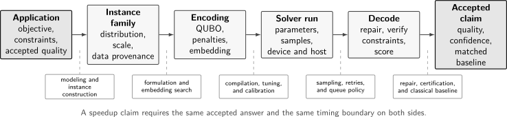
Optimization evidence is end to end only when the same objective, constraints, quality threshold, and timing boundary survive every interface. Omitting embedding search, parameter tuning, failed samples, repair, or the classical baseline can reverse a reported advantage.

Solution Quality Before Speed

Feasibility is not optional

Let $g_a(x)\leq0$ and $h_b(x)=0$ define constraints. The reported solution must be checked against the original formulation, not only the encoded Hamiltonian. A useful feasibility residual is

$$v(x) = \sum_a \left[ \max\{0,g_a(x)\} \right]^2 + \sum_b h_b(x)^2.$$

An infeasible bit string with an excellent penalized energy is not an excellent application solution. If a repair heuristic maps $x$ to $R(x)\in\mathcal F$, the report should give quality and runtime both before and after repair. The repair may be responsible for most of the improvement.

Approximation ratio and optimality gap

For a nonnegative maximization objective, a common approximation ratio is

$$\rho = \frac{ \mathbb E[C_I(X)] }{ C_I(x^\star) }.$$

This is meaningful only when $C_I(x^\star)$ is known and positive. A more general normalized score uses declared reference bounds,

$$\rho_{\mathrm{norm}} = \frac{ \mathbb E[C_I(X)]-C_{\mathrm{worst}} }{ C_{\mathrm{best}}-C_{\mathrm{worst}} }.$$

For an exact solver that supplies a feasible incumbent $C_{\mathrm{inc}}$ and a valid lower bound $L$ for minimization, a relative optimality gap may be

$$g_{\mathrm{rel}} = \frac{ C_{\mathrm{inc}}-L }{ \max\{1,\lvert C_{\mathrm{inc}}\rvert\} }.$$

A heuristic’s best known value is not automatically an optimum. Labels such as “relative accuracy” must say what denominator and reference value were used.

Distributional performance

Optimization heuristics return distributions. Report at least the median, quantiles, and tail behavior over both solver randomness and instance randomness. The expected objective, best-of-$R$ objective, and exact-success probability answer different questions.

If one run succeeds with probability $p_s$, the number of independent runs needed to reach confidence $\eta$ is

$$R_\eta = \left\lceil \frac{ \ln(1-\eta) }{ \ln(1-p_s) } \right\rceil.$$

The corresponding repeated-run time is not simply $R_\eta t_{\mathrm{anneal}}$. It can include reprogramming, state preparation, readout, reset, communication, decoding, and validation.

The Complete Time Boundary

For one instance, a useful ledger is

$$\begin{aligned} T_{\mathrm{total}} ={}& T_{\mathrm{form}} + T_{\mathrm{embed}} + T_{\mathrm{compile}} + T_{\mathrm{tune}} \\ &+ R \left( T_{\mathrm{prepare}} + T_{\mathrm{run}} + T_{\mathrm{read}} \right) \\ &+ T_{\mathrm{repair}} + T_{\mathrm{verify}}. \end{aligned}$$

Cloud queue time may be reported separately from algorithmic wall time, but the policy must be symmetric. A comparison that times only a $20\,\mu\mathrm{s}$ anneal while timing classical parsing, solving, and verification is not end to end. Conversely, a hardware-control benchmark may legitimately exclude application formulation if it excludes equivalent preprocessing for every solver and labels the boundary.

Classical optimizers are often anytime algorithms: given more time, they return progressively better incumbents and bounds. A fair comparison is therefore a quality–time curve,

$$Q_A(t) = \mathbb E_{I\sim\Pi_n} \left[ q_I\!\left( x_A(t) \right) \right],$$

not one quantum point against one prematurely stopped classical run.

Encoding Binary Optimization

QUBO and Ising forms

A quadratic unconstrained binary optimization problem has

$$C(x) = c_0 + \sum_i a_i x_i + \sum_{i<j}b_{ij}x_ix_j, \qquad x_i\in\{0,1\}.$$

With

$$x_i = \frac{1-z_i}{2}, \qquad z_i\in\{-1,+1\},$$

the same objective becomes an Ising energy

$$E(z) = E_0 + \sum_i h_i z_i + \sum_{i<j}J_{ij}z_iz_j.$$

On a gate-model processor, replace $z_i$ by $Z_i$. On an annealer, $h_i$ and $J_{ij}$ are programmed fields and couplings within finite ranges and precision.

Penalties change the landscape

Constraints are often encoded as

$$C_\lambda(x) = C(x) + \sum_a \lambda_a P_a(x), \qquad P_a(x)\geq0.$$

The penalties should guarantee that every encoded optimum is feasible. If $\lambda_a$ is too small, an infeasible state can win. If it is too large, objective differences are compressed relative to hardware precision, noise, or the spectral gap. Penalty selection is part of the algorithm and must not be tuned on hidden test answers.

Connectivity and auxiliary variables

Reducing higher-order terms to quadratic form can introduce ancillas. Embedding a dense logical graph into sparse hardware can represent one logical variable by a connected chain of physical qubits. If $n$ logical variables require $N_{\mathrm{phys}}$ qubits, report the inflation

$$\kappa_{\mathrm{emb}} = \frac{N_{\mathrm{phys}}}{n},$$

the chain-length distribution, embedding-search time, chain strength, and chain-break decoding. A 5,000-qubit machine does not generally accept a fully connected 5,000-variable QUBO.

Case Study 1: QAOA for MaxCut on Sycamore

For a weighted graph $G=(V,E)$, MaxCut assigns $z_i\in\{-1,+1\}$ and maximizes

$$C(z) = \sum_{(i,j)\in E} w_{ij} \frac{1-z_iz_j}{2}.$$

The corresponding cost Hamiltonian is

$$H_C = \sum_{(i,j)\in E} \frac{w_{ij}}{2} \left( I-Z_iZ_j \right).$$

At depth $p$, the standard alternating state is

$$\begin{aligned} \lvert \boldsymbol\gamma,\boldsymbol\beta \rangle ={}& \prod_{\ell=1}^{p} e^{-i\beta_\ell H_B} e^{-i\gamma_\ell H_C} \lvert+\rangle^{\otimes n}, \\ H_B ={}& \sum_iX_i. \end{aligned}$$

This notation is enough to audit the case study; the general variational loop and its optimization errors remain canonical in Variational Quantum Algorithms.

Harrigan and collaborators implemented QAOA on up to 23 superconducting qubits. They compared hardware-native Ising instances with Sherrington–Kirkpatrick and MaxCut instances that required substantial compilation onto the planar processor.

The result cleanly separated two regimes:

• on hardware-native instances, average approximation quality remained roughly stable with size and improved with depth;
• on non-native problems, compilation overhead increased and performance degraded with size;
• circuits containing thousands of gates beat random guessing but did not beat several efficient classical algorithms.

This is a valuable negative-to-mixed case study. It demonstrates coherent algorithmic structure, parameter landscapes, and depth dependence, while showing that graph mismatch can consume the apparent benefit. The relevant resource is compiled two-qubit depth, not the logical QAOA layer count alone.

The experiment also illustrates why random guessing is a weak baseline. MaxCut has strong polynomial-time approximation algorithms, including the Goemans–Williamson semidefinite-programming method with its celebrated worst-case guarantee. Modern exact and heuristic solvers exploit graph structure, preprocessing, local search, branch-and-cut, and parallel hardware. A quantum result should be compared with that portfolio at equal output quality.

Case Study 2: Empirical QAOA Scaling

Low-autocorrelation binary sequences

For spins $s_i\in\{-1,+1\}$, the low-autocorrelation binary sequence problem minimizes

$$C_{\mathrm{LABS}}(s) = \sum_{k=1}^{N-1} \left( \sum_{i=1}^{N-k} s_is_{i+k} \right)^2.$$

Shaydulin and collaborators studied fixed-parameter QAOA for LABS using noiseless simulations up to 40 qubits. Over the fitted range, QAOA time to solution scaled more favorably than the compared branch-and-bound solvers. Combining QAOA with ideal quantum minimum finding gave the strongest empirical scaling in their comparison. They also executed smaller circuits on trapped-ion hardware using algorithm-specific error detection.

The strongest supported label is empirical algorithmic scaling evidence. The fitted QAOA regime was principally noiseless, while the large-scale minimum-finding composition assumes an idealized fault-tolerant quantum computer. Hardware execution demonstrated progress on the circuit family but did not realize the entire favorable-scaling regime end to end.

LABS also has only one canonical instance at each sequence length. That avoids averaging away a hard instance but makes extrapolation sensitive to finite-size irregularities. A mature follow-up should report fit windows, uncertainty in the exponent, alternative classical solvers, total quantum gate cost, and the effect of logical error correction.

One-in-three SAT in 2026

Lu and collaborators introduced a classical restricting-space reduction for positive one-in-three SAT. Mod-2 independent constraints reduce the candidate space from $2^n$ to approximately $2^{n-m}$, and problem-informed quantum ansatzes remain within that reduced space.

Their numerical study compared enhanced QAOA and quantum adiabatic solvers with classical SAT methods on random instances near the critical clause-to-variable ratio. For sizes up to roughly 70 variables, fitted time-to-solution exponents included

$$T_{\mathrm{QAOA}} \propto 1.0077^n, \qquad T_{\mathrm{classical}} \propto 1.0128^n$$

under the paper’s fixed-parameter and solver choices. The reported QAOA circuits used 40 layers in the scaling comparison; the adiabatic reference used 150 layers. A 13-qubit superconducting experiment demonstrated reduced instances originating from problems with 22 variables.

This is newer empirical scaling evidence, not yet a hardware speedup at $n=70$. The classical reduction is a substantive algorithmic contribution and must be included on both sides of a fair comparison where applicable. The authors explicitly leave room for specialized classical heuristics to narrow the fitted gap. The result is therefore promising and testable: increase the executed range, publish full timing, test broader instance ensembles, and continue the classical solver search.

What a fitted exponent does and does not show

Suppose two empirical times are fit as

$$T_Q(n) \approx A\alpha^n, \qquad T_C(n) \approx B\beta^n, \qquad \alpha<\beta.$$

The crossover is

$$n_\times = \frac{ \ln(A/B) }{ \ln(\beta/\alpha) }.$$

A favorable exponent can coexist with an inaccessible crossover if $A/B$ is large. Exponent uncertainty, fit-window choice, hidden polynomial factors, noise scaling, and a new classical algorithm can all move $n_\times$. Scaling evidence is stronger than a one-size prefactor win, but it is not a complexity theorem.

Case Study 3: Rydberg Maximum Independent Set

For a graph $G=(V,E)$, an independent set has binary variables $x_i\in\{0,1\}$ satisfying

$$x_i+x_j \leq 1 \qquad \text{for every }(i,j)\in E.$$

Maximum independent set maximizes

$$C(x) = \sum_{i\in V} w_i x_i.$$

In a neutral-atom array, vertices are represented by atoms and nearby simultaneous Rydberg excitations are energetically suppressed. A typical Hamiltonian is

$$H(t) = \frac{\hbar\Omega(t)}{2} \sum_iX_i - \hbar\Delta(t) \sum_i n_i + \sum_{i<j} V_{ij}n_in_j.$$

When graph edges match the blockade geometry, the hardware provides a direct encoding of unit-disk-graph independent sets.

Ebadi and collaborators used arrays of up to 289 atoms, closed-loop schedule optimization, and deep coherent evolution. On selected hard graph families, they reported superlinear scaling relative to their simulated-annealing baseline for finding exact solutions.

This was an important scale and control result, but the baseline conclusion was not final. Andrist and collaborators tested broader exact and heuristic classical methods. They found that the quasi-planar Union-Jack-like instances could be solved to optimality for thousands of vertices within minutes on commodity hardware, and that a less restricted simulated-annealing implementation was competitive with the quantum protocol. They also identified less structured, higher-connectivity instances that were much harder and proposed them as stronger future tests.

The pair of studies is exemplary scientific progress:

1. a quantum experiment identifies a candidate scaling regime;
2. classical researchers exploit previously underused structure;
3. the apparent frontier moves;
4. better instance families and protocols are proposed.

The correct conclusion is not that the hardware result disappeared. The experiment still demonstrated 289-atom programmable optimization and mechanism-level behavior. What changed was the strength of the speedup claim.

Finite blockade, long-range interaction tails, atom loss, and readout errors can produce strings outside the intended independent-set space. Reports should therefore give raw feasibility, repair policy, post-repair quality, and all discarded samples. Extending arbitrary graphs with quantum wires or auxiliary atoms can enlarge the instance class, but the added atoms and smaller energy scales belong in the resource count.

Case Study 4: Superconducting Quantum Annealing

Physical process

A transverse-field annealer implements a time-dependent Hamiltonian such as

$$H(s) = -A(s) \sum_iX_i + B(s) \left( \sum_i h_iZ_i + \sum_{i<j}J_{ij}Z_iZ_j \right),$$

where $s$ increases from $0$ to $1$. In an ideal closed-system adiabatic limit, a sufficiently slow schedule can follow the ground state. The required runtime depends on spectral gaps and matrix elements and can grow rapidly with problem size. Real devices are open, finite-temperature systems with control error and a minimum programmable anneal time.

Adiabatic Quantum Computation owns the ideal closed-system Hamiltonian-path model, including its accepted subspace, decoder, schedule, error certificate, and logical resources. This case study retains the open-system device evidence, time-to-solution boundaries, instance ensembles, and matched speedup baselines; quantum annealing is not identified with universal AQC.

Quantum Annealing supplies the device-agnostic finite-time process record for the driver–problem path, closed or reduced-open regime, thermal and freeze-out assumptions, decoded sample distribution, embeddings, gauges, repetitions, and annealing resources. This case study continues to own whether that process solves the declared application competitively.

Evidence that a device exhibits quantum annealing is not the same as evidence of computational speedup. Boixo and collaborators found that a 108-qubit device correlated with simulated quantum annealing more strongly than with simple classical spin dynamics. Rønnow and collaborators formalized several speedup notions and showed why the conclusion depends on the classical comparison class and timing boundary.

Crafted tunneling instances

Denchev and collaborators designed weak–strong cluster instances with tall, narrow barriers. A D-Wave 2X annealer showed large prefactor advantages over single-core simulated annealing and quantum Monte Carlo for the chosen comparison. The authors also noted that structure-aware classical solvers could solve most Chimera-structured instances on comparable timescales. Subsequent work catalogued those strengths and weaknesses.

The narrow claim is limited quantum speedup relative to selected corresponding classical annealing methods on crafted instances. It is not strong quantum speedup over every classical algorithm, and it is not a practical application advantage. Crafted benchmarks are useful when they isolate tunneling, but an application must show that the same favorable landscape arises without constructing the problem around the hardware.

Large hybrid-QUBO studies

A 2025 benchmarking study compared D-Wave quantum and hybrid services with a set of classical solvers on dense QUBOs up to 10,000 variables. It reported very large time advantages and slightly better solution values for the hybrid service under its chosen solver set and timing definitions.

The largest problems could not fit directly on the QPU. They were handled by QUBO decomposition or a hybrid quantum–classical service. The result should therefore be labeled a solver-stack benchmark, not a pure-QPU speedup. Because the hybrid service is itself a classical–quantum algorithm, causal attribution requires ablations: classical host alone, identical decomposition with and without quantum calls, equal tuning, equal stopping, and full access to timing and solver settings. “Best value seen” is not an optimality certificate when the optimum is unknown.

Speedup vocabulary

Useful labels include:

Label	Comparison
quantum process evidence	device behavior is inconsistent with selected classical physical models
limited quantum speedup	quantum implementation beats classical versions of the same annealing approach
potential quantum speedup	quantum solver beats a specified portfolio of classical algorithms
strong quantum speedup	quantum solver beats the best possible classical algorithm under a defensible complexity model
practical advantage	quantum workflow returns accepted application answers with lower end-to-end cost than the dated best alternative

The first two labels do not imply the last two.

Case Study 5: Grover-Based Optimization

Minimum finding

If an objective can be queried coherently over $N$ candidates, Dürr–Høyer minimum finding uses an expected

$$O(\sqrt N)$$

objective-oracle calls, compared with $\Theta(N)$ evaluations for unstructured classical search. This is a genuine asymptotic quadratic query speedup.

The oracle is not free. A reversible comparison must:

1. construct or load the candidate;
2. test all constraints;
3. evaluate the objective to sufficient precision;
4. compare with a threshold;
5. uncompute temporary data.

If one oracle call costs $G_f$ fault-tolerant gates, the useful leading resource is of order

$$G_{\mathrm{search}} \sim G_f\sqrt N,$$

plus state preparation, threshold updates, error correction, and repeated success amplification. A classical algorithm that exploits problem structure may examine far fewer than $N$ leaves.

Backtracking and branch-and-bound

Quantum walks can quadratically accelerate broad classes of backtracking trees under explicit access assumptions. Quantum branch-and-bound similarly offers approximately square-root dependence on explored tree size, with additional factors for depth, bound evaluation, and error probability.

These algorithms are more relevant to structured optimization than flat Grover search because they preserve classical pruning. Their practical questions are:

• can the branching and bound procedures be made reversible at reasonable depth?
• how much memory and data access are required?
• is the classical tree size known or estimated without solving the instance?
• does the quantum algorithm return a witness, a bound, or only a decision?
• what classical parallelism is the comparison allowed?

Campbell, Khurana, and Montanaro compiled Grover and quantum-backtracking approaches for random SAT and graph coloring into fault-tolerant estimates. They found potentially large speedups under optimistic and conservative assumptions, but also extremely large physical-qubit requirements. In their least favorable accounting, classical surface-code decoding could erase the advantage. This is an unusually valuable resource case because it exposes oracle construction and fault-tolerance overhead instead of stopping at $O(\sqrt N)$.

Case Study 6: Structured Interference Beyond Grover

Decoded quantum interferometry uses quantum Fourier transforms and reversible decoders to bias samples toward high-quality objective values. Jordan and collaborators proved a superpolynomial separation from known classical algorithms for a structured polynomial-fitting problem over finite fields. For sparse max-XORSAT, their DQI construction beat several general-purpose heuristics, while a tailored classical solver later built for that instance performed better.

The distinction is instructive:

• the structured polynomial-fitting result is an algorithmic separation relative to known algorithms under a specified average-case setting;
• the max-XORSAT experiment is evidence that Fourier and decoding structure can guide optimization, not an advantage demonstration;
• a proposed instance around 521 field elements required an estimate of about $10^8$ logical Toffoli gates and $9\times10^3$ logical qubits for a key reversible decoder, so the result is fault-tolerant rather than near-term.

DQI broadens the design space beyond Hamiltonian heuristics. It also reinforces the central lesson of every case study: once an instance reveals exploitable structure, classical algorithm development must be invited rather than frozen.

Benchmark Design That Survives Contact

Use a portfolio, not a mascot baseline

Depending on the problem, include:

• exact mixed-integer programming with incumbent and bound;
• branch-and-cut, branch-and-price, constraint programming, or SAT;
• semidefinite and linear relaxations;
• problem-specific approximation algorithms;
• local search, tabu search, simulated annealing, parallel tempering, and large-neighborhood search;
• tensor-network or dynamic-programming methods for favorable graph width;
• GPU QUBO heuristics and quantum-inspired solvers;
• ablated hybrid pipelines.

Give every method comparable tuning budgets and hardware information. A single off-the-shelf simulated-annealing implementation is rarely “classical optimization.”

Choose instances before outcomes

Publish the generator, seeds, feature distributions, planted structure, and selection rule. Split development and test sets. Avoid choosing the instances where one solver happened to look best. Include easy controls, crossover instances, and classically hard instances with independently established difficulty.

The 2026 Quantum Optimization Benchmarking Library provides ten model-independent problem classes, versioned instances, known or best-known solutions, and classical baselines. Such shared sets do not settle advantage, but they reduce private-instance selection and make future improvements auditable.

Separate training from evaluation

If parameters, schedules, penalties, embeddings, or repair rules are trained on instances, report the training cost and evaluate on held-out instances. Parameter transfer can be a valid algorithmic feature; tuning on the exact test answer is leakage.

Preserve the application objective

An industrial label does not make a QUBO industrial. Report which original constraints and costs were retained, approximated, or dropped. Compare the decoded solution with the organization’s actual incumbent method and include the cost of turning a bit string into an actionable schedule or design.

Common Mistakes

“The problem is NP-hard, so this instance is hard”

NP-hardness is a worst-case statement about a problem family. Structured, small, low-density, low-treewidth, or planted instances may be easy.

“More qubits means a larger logical problem”

Ancillas, chains, gauge copies, slack variables, and wires can consume most physical qubits. Report the original decision-variable count and all encoding inflation.

“The anneal time is the runtime”

Programming, embedding, gauges, reads, reset, network latency, decoding, and repetition can dominate a microsecond-scale anneal.

“The lowest energy sample is the best solution”

Only after mapping back to original variables, checking feasibility, undoing offsets and penalties, and evaluating the original objective.

“A favorable fitted exponent proves asymptotic speedup”

Finite-range scaling is evidence. It is sensitive to prefactors, fit windows, noise, instance distribution, and the classical solver frontier.

“QAOA beating random guessing shows usefulness”

Random guessing ignores efficient approximation algorithms and modern heuristics. It is a sanity check, not a practical baseline.

“Hybrid means quantum-enhanced”

A hybrid service may be excellent software while deriving its performance mainly from classical decomposition and local search. Ablations are required to attribute improvement to quantum calls.

“Best known means optimal”

When no certificate exists, report a lower or upper bound, best-known provenance, and gap. Do not compute a misleading percentage accuracy from an uncertified denominator.

A Reproducible Optimization Report

For every case study, publish:

1. Application contract: original data, constraints, objective, and accepted quality.
2. Instance contract: distribution, generator, seeds, sizes, features, development/test split, and known bounds.
3. Encoding: QUBO or Hamiltonian coefficients, penalties, ancillas, scaling, precision, and embedding.
4. Quantum protocol: device, calibration, circuit or schedule, compilation, shots, gauges, postselection, mitigation, and failures.
5. Hybrid control: optimizer, initialization, stopping, parameter history, host hardware, and total quantum calls.
6. Decoding: chain-break policy, repair, feasibility, and original objective recomputation.
7. Metrics: distributions of quality and time, confidence intervals, exact-success probability, and bound gaps.
8. Baselines: solver versions, settings, tuning budgets, hardware, parallelism, and convergence evidence.
9. Artifacts: raw samples, code, logs, embeddings, timing traces, and versioned result tables.

Reporting Standards owns the full provenance requirements. Resource Estimation Tools owns logical-to-physical compilation for fault-tolerant search.

Current Evidence

As of August 2026:

1. QAOA has substantial algorithmic evidence but no general practical advantage. Hardware experiments reveal depth, connectivity, and noise behavior. LABS and one-in-three SAT studies provide meaningful empirical scaling evidence, chiefly in ideal or noiseless regimes with smaller hardware demonstrations.
2. Analog Rydberg optimization operates at hundreds of atoms. Direct geometric encoding is compelling, but stronger classical baselines revised the interpretation of the first reported MIS scaling advantage.
3. Quantum annealers exhibit quantum dynamics and can be strong heuristic components. Limited speedups and favorable solver-stack comparisons are documented. Strong or practical advantage remains dependent on benchmark, baseline, decomposition, and timing boundaries.
4. Grover-based methods offer rigorous quadratic query improvements. Oracle construction, fault tolerance, and strong classical pruning determine whether those improvements become wall-clock gains.
5. Structured algorithms are expanding the frontier. DQI and problem-informed reductions show that optimization algorithms need not be generic energy minimizers, but their most ambitious resource requirements are fault-tolerant.
6. No broadly accepted end-to-end practical quantum advantage on a useful optimization application has yet been established. The most credible path combines shared hard instances, complete timing, held-out evaluation, strong evolving baselines, and a quantum protocol executable in the fitted scaling regime.

That conclusion does not reduce all current work to failure. Negative results identify compilation and baseline bottlenecks; scaling studies create falsifiable targets; and shared benchmark libraries make future advantage claims substantially more trustworthy.

Related Pages

• Grover Search derives query-optimal unstructured search and its oracle assumptions.
• Variational Quantum Algorithms develops hybrid-loop cost, trainability, gradients, and validation.
• Why Benchmarking Is Hard explains workload dependence, moving baselines, and metric gaming.
• Verification of Quantum Advantage defines computational, practical, and scientific advantage claims.
• Algorithmic Benchmarking owns accepted-answer boundaries and matched time to solution.
• Resource Estimation Tools develops versioned fault-tolerant estimate bundles.
• Negative Results and Limitations classifies reachability bounds, empirical nulls, baseline reversals, and open practical-advantage claims without conflating them.

References

1. E. Farhi, J. Goldstone, and S. Gutmann, “A quantum approximate optimization algorithm,” arXiv:1411.4028 (2014), doi:10.48550/arXiv.1411.4028.
2. S. Hadfield et al., “From the quantum approximate optimization algorithm to a quantum alternating operator ansatz,” Algorithms 12, 34 (2019), doi:10.3390/a12020034.
3. M. X. Goemans and D. P. Williamson, “Improved approximation algorithms for maximum cut and satisfiability problems using semidefinite programming,” Journal of the ACM 42, 1115–1145 (1995), doi:10.1145/227683.227684.
4. M. P. Harrigan et al., “Quantum approximate optimization of non-planar graph problems on a planar superconducting processor,” Nature Physics 17, 332–336 (2021), doi:10.1038/s41567-020-01105-y.
5. R. Shaydulin et al., “Evidence of scaling advantage for the quantum approximate optimization algorithm on a classically intractable problem,” Science Advances 10, eadm6761 (2024), doi:10.1126/sciadv.adm6761.
6. Q. Lu et al., “Evidence of scaling advantage on an NP-complete problem with enhanced quantum solvers,” Nature Computational Science (2026), doi:10.1038/s43588-026-01007-8.
7. S. Ebadi et al., “Quantum optimization of maximum independent set using Rydberg atom arrays,” Science 376, 1209–1215 (2022), doi:10.1126/science.abo6587.
8. R. S. Andrist et al., “Hardness of the maximum independent set problem on unit-disk graphs and prospects for quantum speedups,” Physical Review Research 5, 043277 (2023), doi:10.1103/PhysRevResearch.5.043277.
9. T. Kadowaki and H. Nishimori, “Quantum annealing in the transverse Ising model,” Physical Review E 58, 5355–5363 (1998), doi:10.1103/PhysRevE.58.5355.
10. T. Albash and D. A. Lidar, “Adiabatic quantum computation,” Reviews of Modern Physics 90, 015002 (2018), doi:10.1103/RevModPhys.90.015002.
11. S. Boixo et al., “Evidence for quantum annealing with more than one hundred qubits,” Nature Physics 10, 218–224 (2014), doi:10.1038/nphys2900.
12. T. F. Rønnow et al., “Defining and detecting quantum speedup,” Science 345, 420–424 (2014), doi:10.1126/science.1252319.
13. V. S. Denchev et al., “What is the computational value of finite-range tunneling?” Physical Review X 6, 031015 (2016), doi:10.1103/PhysRevX.6.031015.
14. S. Mandrà et al., “Strengths and weaknesses of weak-strong cluster problems: a detailed overview of state-of-the-art classical heuristics versus quantum approaches,” Physical Review A 94, 022337 (2016), doi:10.1103/PhysRevA.94.022337.
15. S. Kim et al., “Quantum annealing for combinatorial optimization: a benchmarking study,” npj Quantum Information 11, 77 (2025), doi:10.1038/s41534-025-01020-1.
16. L. K. Grover, “A fast quantum mechanical algorithm for database search,” in Proceedings of the Twenty-Eighth Annual ACM Symposium on Theory of Computing, 212–219 (1996), doi:10.1145/237814.237866.
17. C. Dürr and P. Høyer, “A quantum algorithm for finding the minimum,” arXiv:quant-ph/9607014 (1996), doi:10.48550/arXiv.quant-ph/9607014.
18. A. Montanaro, “Quantum-walk speedup of backtracking algorithms,” Theory of Computing 14, 1–24 (2018), doi:10.4086/toc.2018.v014a015.
19. A. Montanaro, “Quantum speedup of branch-and-bound algorithms,” Physical Review Research 2, 013056 (2020), doi:10.1103/PhysRevResearch.2.013056.
20. E. Campbell, A. Khurana, and A. Montanaro, “Applying quantum algorithms to constraint satisfaction problems,” Quantum 3, 167 (2019), doi:10.22331/q-2019-07-18-167.
21. S. P. Jordan et al., “Optimization by decoded quantum interferometry,” Nature 646, 831–836 (2025), doi:10.1038/s41586-025-09527-5.
22. T. Koch et al., “The Quantum Optimization Benchmarking Library,” Nature Computational Science 6, 653–671 (2026), doi:10.1038/s43588-026-00991-1.
23. A. Abbas et al., “Challenges and opportunities in quantum optimization,” Nature Reviews Physics 6, 718–735 (2024), doi:10.1038/s42254-024-00770-9.
24. G. G. Guerreschi and A. Y. Matsuura, “QAOA for Max-Cut requires hundreds of qubits for quantum speed-up,” Scientific Reports 9, 6903 (2019), doi:10.1038/s41598-019-43176-9.
25. J. Wurtz and D. Lykov, “Fixed-angle conjectures for the quantum approximate optimization algorithm on regular MaxCut graphs,” Physical Review A 104, 052419 (2021), doi:10.1103/PhysRevA.104.052419.
26. S. Yarkoni et al., “Quantum annealing for industry applications: introduction and review,” Reports on Progress in Physics 85, 104001 (2022), doi:10.1088/1361-6633/ac8c54.
27. D. Venturelli et al., “Quantum optimization of fully connected spin glasses,” Physical Review X 5, 031040 (2015), doi:10.1103/PhysRevX.5.031040.

Exercises

1. Compute a repeated-run time

One solver call succeeds with probability $p_s=0.02$ and takes $4\,\mathrm{ms}$ including preparation and readout. Programming costs $0.8\,\mathrm{s}$ once. Find the number of calls and total time required for $99\%$ success, ignoring all other costs.

Solution

The repetition count is

$$R_{0.99} = \left\lceil \frac{\ln(0.01)}{\ln(0.98)} \right\rceil = 228.$$

The repeated calls take

$$228 \left( 4\,\mathrm{ms} \right) = 0.912\,\mathrm{s}.$$

Including one programming step gives

$$T_{\mathrm{total}} = 0.8+0.912 = 1.712\,\mathrm{s}.$$

Timing only the $4\,\mathrm{ms}$ call would understate time to the accepted answer by more than two orders of magnitude.

2. Convert a QUBO term

Map $3x_1x_2-2x_1$ to Ising variables using $x_i=(1-z_i)/2$.

Solution

First,

$$3x_1x_2 = \frac34 \left( 1-z_1-z_2+z_1z_2 \right),$$

and

$$-2x_1 = -1+z_1.$$

Therefore

$$3x_1x_2-2x_1 = -\frac14 + \frac14z_1 - \frac34z_2 + \frac34z_1z_2.$$

The constant does not change the minimizing bit string but must be restored when comparing absolute objective values.

3. Choose a penalty

The feasible objective lies between $0$ and $20$. One constraint penalty is $P(x)=0$ for feasible strings and $P(x)\geq1$ otherwise. Give a sufficient penalty weight for minimization and explain why an arbitrarily huge value may still be undesirable.

Solution

Any $\lambda>20$ is sufficient if infeasible objective values can be as low as zero and every feasible objective is at most $20$: every infeasible penalized value then exceeds every feasible one. A tighter bound may be possible with more objective information.

An extremely large $\lambda$ expands coefficient range. Rescaling to hardware limits then compresses distinctions among feasible solutions, making them more sensitive to coefficient quantization, control error, and noise. Large penalties can also reduce useful spectral gaps.

4. Find a scaling crossover

Suppose

$$T_Q(n)=10^6(1.008)^n$$

and

$$T_C(n)=(1.013)^n.$$

Estimate the crossover size.

Solution

Set the times equal:

$$10^6 \left( \frac{1.008}{1.013} \right)^n = 1.$$

Thus

$$n = \frac{\ln(10^6)}{\ln(1.013/1.008)} \approx 2812.$$

The favorable quantum exponent does not help at accessible sizes under this large prefactor. Small changes in either fitted base can move the crossover substantially.

5. Audit an approximation ratio

A maximization paper reports a best sample of $92$, calls $100$ the optimum, and quotes $\rho=0.92$. Later, a classical solver finds value $106$. What was wrong, and what can still be reported?

Solution

The denominator was an uncertified best-known value, not the optimum. The claimed approximation ratio was therefore invalid. The paper can report the raw feasible value $92$, its gap to a valid upper bound if one exists, and its ratio to the contemporaneous best known value with that narrower label. Against the later incumbent, the simple value ratio is

$$\frac{92}{106} \approx 0.868,$$

but this is still not an approximation ratio to the true optimum unless $106$ is certified optimal.

6. Diagnose embedding inflation

A complete 60-variable QUBO uses 1,770 quadratic couplings. An embedding requires 1,140 physical qubits. Find the inflation factor and list two additional quantities needed to evaluate the embedding.

Solution

The inflation is

$$\kappa_{\mathrm{emb}} = \frac{1140}{60} = 19.$$

The report should also give the chain-length distribution, chain strength, embedding-search time, coefficient rescaling, chain-break rate, decoding policy, and post-decoding feasibility. Any two of these answer the question.

7. Compare flat search with pruning

An optimization space has $N=2^{80}$ candidates. A classical branch-and-bound solver explores $2^{30}$ leaves on the instance. Compare ideal Grover search over the full space with a square-root acceleration of the explored tree.

Solution

Flat Grover search needs order

$$\sqrt{2^{80}} = 2^{40}$$

oracle calls. A quantum backtracking or branch-and-bound method with ideal square-root dependence on the classical tree would need order

$$\sqrt{2^{30}} = 2^{15}$$

tree operations, up to algorithmic factors. Preserving classical structure is exponentially better on this instance than pretending the search space is unstructured. Reversible branching, bounds, and memory still have to be costed.

8. Design an ablation for a hybrid solver

A proprietary hybrid annealing service beats four classical heuristics on large QUBOs. Propose the minimum ablation needed to attribute the result to quantum processing.

Solution

Run the identical outer decomposition, initialization, stopping rule, tuning budget, repair, and host hardware with the quantum subproblem calls replaced by strong classical subproblem solvers. Also compare QPU-only subproblems where they fit, record every quantum and classical call, and include end-to-end timing and quality distributions. Attribution requires a statistically significant improvement from quantum calls over these matched ablations; superiority of the opaque whole service does not identify the responsible component.