QAOA

QAOA is a family of parameterized quantum states built by alternating an objective-dependent phase separator with a mixer. This page uses one maximization convention throughout: larger eigenvalues of the diagonal cost operator $C$ are better, and the circuit applies $U_C(\gamma)=e^{-i\gamma C}$ before $U_B(\beta)=e^{-i\beta B}$ in each layer. The original construction is the quantum approximate optimization algorithm of Farhi, Goldstone, and Gutmann (2014); constrained and more general variants are often called the quantum alternating operator ansatz. The ansatz supports exact finite-depth analysis and useful family-specific results, but neither its form nor any result below establishes a generic end-to-end practical speedup over classical optimization.

Required background. Variational Quantum Algorithms supplies the hybrid optimization loop, objective and gradient estimators, and the independent-validation discipline used here.

Helpful background. Circuit Model supplies gate order and resource conventions; Pauli Matrices supplies Pauli exponentials; Adiabatic Quantum Computation supplies closed-system interpolation semantics; and Optimization Case Studies owns dated experiments and practical comparisons.

QAOA as Alternating Cost-and-Mixer Dynamics

Let a classical score $C(z)$ be assigned to each $n$-bit string. Its diagonal operator and the standard transverse-field mixer are

$$C=\sum_z C(z)\lvert z\rangle\langle z\rvert, \qquad B=\sum_{j=1}^{n}X_j.$$

The corresponding unitaries are

$$U_C(\gamma)=e^{-i\gamma C}, \qquad U_B(\beta)=e^{-i\beta B}.$$

$U_C$ changes phases according to objective value but leaves computational-basis probabilities unchanged. $U_B$ then mixes amplitudes between strings that differ in one bit. Alternating the two can turn relative phases into a probability bias toward high-scoring strings. That interference mechanism is more precise than saying that the circuit “searches all answers at once”: useful bias depends on the encoded objective, initial state, mixer, angles, and depth.

“QAOA” is used for three related objects that should not be conflated. The original quantum approximate optimization algorithm uses a cost operator, the transverse-field mixer, the uniform initial state, and shared angles at a fixed level $p$. The broader quantum alternating operator ansatz replaces the initial state, phase separator, or mixer to encode constraints and problem structure, as formalized by Hadfield et al. (2019). A Hamiltonian variational ansatz alternates physically motivated noncommuting Hamiltonian terms and may target a quantum state rather than a classical bit string; early examples appear in Wecker, Hastings, and Troyer (2015). The last usage is QAOA-like, but a computational-basis measurement is not generally an energy sample for a non-diagonal target Hamiltonian.

The state family is only one part of an algorithm. An executable procedure also chooses a level, generates or transfers initial angles, allocates an optimization budget, compiles and executes every requested circuit, estimates scores, selects a checkpoint, validates it with fresh shots, samples candidate solutions, checks feasibility, decodes them, and applies a retry rule. Omitting those operations changes both the scientific claim and its cost.

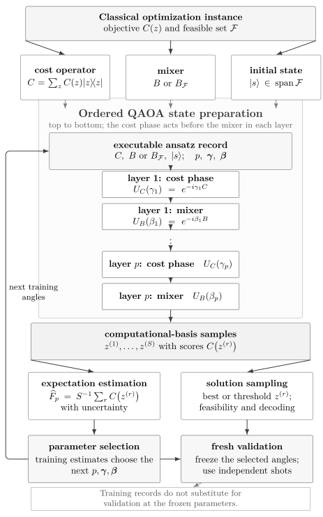
The ordered cost-and-mixer layers define the state family. Parameter selection, measurement allocation, solution decoding, and fresh validation are part of the executable algorithm; expectation estimation and solution sampling are distinct outputs.

The Ten-Field QAOA Claim Record

A performance statement becomes auditable only after its task, interfaces, output, costs, comparator, and evidence are fixed. The following record instantiates the chapter-wide ten-field contract for one family: unweighted MaxCut on explicitly listed simple triangle-free $d$-regular graphs. It is a specification, not a claim that this family is hard or practically useful.

Field	Required declaration
Problem family and size	Unweighted MaxCut on a simple triangle-free $d$-regular graph $G=(V,E)$, with $n=\lvert V\rvert$ and $m=\lvert E\rvert$.
Promise and instance	Adjacency lists are validated as simple, undirected, triangle-free, and $d$-regular; the named graph and vertex ordering are archived.
Access and encoding	The full edge list is classical input; one qubit encodes each vertex, $x_i=(I-Z_i)/2$, edge weights are one, and the cost has no omitted offset.
Output and use	The procedure returns measured bitstrings, their cut values, and the best validated string; complementary strings encode the same cut.
Success and error	Report fresh-shot $F_p$, its interval, feasibility probability, and a prespecified threshold-hit probability; do not substitute one metric for another.
Algorithmic idea	Prepare $\lvert+\rangle^{\otimes n}$ and alternate the diagonal MaxCut separator with $B=\sum_iX_i$ for a declared level $p$.
Executable procedure	Prespecify angle initialization or transfer, optimizer and parameter-search budget, seeds, stopping rule, shot allocation, selected checkpoint, validation set, decoder, and retries.
Resource ledger	Record compilation and routing, $p$, all objective or gradient calls, logical and compiled gates, depth, shots, rejected runs, calibration, mitigation, decoding, and wall-clock time.
Classical comparator	Use a dated exact or heuristic portfolio, and the Goemans–Williamson relaxation where appropriate, on the identical graph and output criterion with matched total-cost boundaries.
Evidence and limits	Bound conclusions to the tested family, sizes, optimizer budget, compilation, and noise model; an ideal depth-one formula validates analysis but proves no generic practical advantage.

Several fields deliberately repeat quantities that a circuit diagram hides. For example, “$p=3$” does not state how many parameter points were evaluated, how many shots each point received, how many seeds failed, which compiled two-qubit gates were executed, or how a returned bitstring was accepted. The Algorithmic Benchmarking page owns the general execution record, while Resource Estimation Tools owns logical-to-physical translation. A QAOA result should carry both records rather than replace them with nominal layer count.

From a Classical Objective to a Cost Hamiltonian

Binary variables and diagonal operators

For $x_i\in\{0,1\}$, the computational-basis eigenvalue relation $Z_i\lvert x_i\rangle=(-1)^{x_i}\lvert x_i\rangle$ gives

$$x_i\mapsto\frac{I-Z_i}{2}, \qquad x_ix_j\mapsto \frac{I-Z_i-Z_j+Z_iZ_j}{4}.$$

Thus a quadratic unconstrained binary objective

$$f(x)=c+\sum_i h_i x_i+\sum_{i<j}Q_{ij}x_ix_j$$

becomes an Ising operator containing a constant, one-body $Z_i$ terms, and two-body $Z_iZ_j$ terms. The substitution is an equality on every basis state, not a continuous relaxation. Higher-degree monomials similarly become products of diagonal Pauli operators, although reducing their locality may require ancillas and penalties whose costs belong in the encoding.

Here the quadratic sum is over distinct variables. If a QUBO matrix notation includes diagonal terms, reduce them first with $x_i^2=x_i$ and absorb their coefficients into the linear terms before applying the two-variable substitution.

For weighted MaxCut, an edge $\{u,v\}$ is cut exactly when the endpoint bits differ. Its indicator is

$$x_u+x_v-2x_ux_v = \frac12(I-Z_uZ_v),$$

so, for weights $w_{uv}$,

$$C = \sum_{\{u,v\}\in E} \frac{w_{uv}}{2}(I-Z_uZ_v).$$

Every term is diagonal and all terms commute. Consequently,

$$U_C(\gamma) = \prod_{\{u,v\}\in E} \exp\!\left[-\frac{i\gamma w_{uv}}{2}(I-Z_uZ_v)\right]$$

is an exact factorization. Calling it a Trotter approximation would introduce an error that is absent. A compiler may discard the product of constant-term phases, but it must retain the coefficient scale that determines the useful angle and the physical rotation precision.

Penalties and objective scale

Constraints can be encoded by maximizing

$$C_\lambda=C-\lambda P,$$

where $P=0$ on feasible strings and $P\ge1$ on infeasible strings. If the unpenalized objective is bounded by $C_{\min}\le C(z)\le C_{\max}$ on all strings, then the crude sufficient condition

$$\lambda>C_{\max}-C_{\min}$$

makes every infeasible penalized value at most $C_{\max}-\lambda<C_{\min}$, whereas every feasible value is at least $C_{\min}$. This condition is sufficient, not necessary. A tighter problem-specific gap can permit a much smaller penalty. Large coefficients expand the phase range, demand finer control, can worsen objective-estimation variance, and may require additional high-locality decomposition or ancillas. “Unconstrained” in QUBO therefore does not mean cost-free encoding.

Affine changes also require care. For

$$C'=\alpha C+\kappa I,$$

the identity contribution produces only the global phase $e^{-i\gamma\kappa}$, while $\alpha$ rescales the effective angle from $\gamma$ to $\alpha\gamma$. It is safe to drop $\kappa I$ during state preparation if its value is restored when reporting the original objective. It is not safe to assume an approximation ratio is shift invariant: $F/C_{\max}$ and $(F+\kappa)/(C_{\max}+\kappa)$ are generally different. The report must state offsets, normalization, and whether the metric is a raw expectation, normalized score, or ratio to a known optimum.

The Standard Depth-p Circuit

Shared angles and operator order

At level $p$, the declared state is

$$\lvert\boldsymbol\gamma,\boldsymbol\beta\rangle = U_B(\beta_p)U_C(\gamma_p)\cdots U_B(\beta_1)U_C(\gamma_1)\lvert s\rangle.$$

The rightmost operation acts first. The standard unconstrained construction uses

$$\lvert s\rangle=\lvert+\rangle^{\otimes n},$$

so the phase separator acts on a uniform superposition before the mixer in each layer. There are $2p$ shared real parameters: every cost term uses the same $\gamma_\ell$ and every mixer term uses the same $\beta_\ell$ within layer $\ell$. Parameter sharing is part of the ansatz and is distinct from a more general circuit that assigns an angle to each edge or vertex.

The maximization signs matter. Authors who minimize a problem Hamiltonian, define $e^{+i\gamma C}$, reverse the mixer sign, or write products in the opposite order obtain angle formulas related by sign changes or reordered coordinates. Transcribing a reported optimum without transcribing its generator and order conventions is therefore unsafe.

The ideal expectation and output distribution are

$$F_p(\boldsymbol\gamma,\boldsymbol\beta) = \langle C\rangle = \sum_z C(z)P_p(z),$$ $$P_p(z) = \left\lvert \langle z\vert\boldsymbol\gamma,\boldsymbol\beta\rangle \right\rvert^2.$$

$F_p$ is an average score. It is not the probability of sampling an optimum, nor does it determine the whole tail of $P_p$. Two angle sets can have the same expectation but very different probabilities of returning a usable candidate. The hybrid algorithm must therefore optimize and validate the metric that matches the declared output use.

MaxCut at p = 1

The general depth-one edge formula

Consider unweighted MaxCut on a simple graph under the exact convention above, with $\lvert s\rangle=\lvert+\rangle^{\otimes n}$ and $p=1$. For an edge $(u,v)$, let

$$a=\deg(u)-1, \qquad b=\deg(v)-1,$$

and let $\lambda$ be the number of triangles containing that edge. Then the ideal expected contribution of $C_{uv}=(I-Z_uZ_v)/2$ is

$$\begin{aligned} \langle C_{uv}\rangle ={}&\frac12+ \frac14\sin(4\beta)\sin\gamma \left(\cos^a\gamma+\cos^b\gamma\right)\\ &-\frac14\sin^2(2\beta) \cos^{a+b-2\lambda}\gamma \left[1-\cos^\lambda(2\gamma)\right]. \end{aligned}$$

The result follows by evaluating the edge observable in the Heisenberg picture. Mixer conjugation sends each endpoint $Z$ into a linear combination of $Z$ and $Y$ with angle $2\beta$. Cost terms incident on one endpoint rotate the resulting $Y$ into $X$ components. Expectation in the plus state removes every Pauli string containing a remaining $Y$ or $Z$. Neighbors unique to one endpoint supply powers of $\cos\gamma$; common neighbors create paired paths whose interference produces the final triangle term. Terms outside the radius-one edge neighborhood cancel from this local expectation.

This formula, derived in the depth-one MaxCut analysis of Wang et al. (2018), is easy to quote incorrectly. The last term vanishes only when $\lambda=0$ (or at special angles), so the triangle-free expression cannot be applied to a graph merely because it is regular. The hypotheses also exclude weighted edges unless the angle dependence is rederived with each incident weight.

For one isolated edge, $a=b=\lambda=0$, and the expression reduces to

$$\langle C_{uv}\rangle = \frac12+\frac12\sin(4\beta)\sin\gamma.$$

At $\beta=\pi/8$ and $\gamma=\pi/2$, the cut expectation is one. The finite audit below verifies the stronger statement that all probability lies on the two cut bitstrings.

Triangle-free regular graphs

For a simple triangle-free $d$-regular graph with $d\ge2$, every edge has $a=b=d-1$ and $\lambda=0$. Summing identical edge expectations gives

$$\frac{F_1}{\lvert E\rvert} = \frac12+ \frac12\sin(4\beta)\sin\gamma\cos^{d-1}\gamma.$$

Choose the positive branch. The factor $\sin(4\beta)$ is maximized by $\beta=\pi/8$. For $g(\gamma)=\sin\gamma\cos^{d-1}\gamma$,

$$g'(\gamma) = \cos^{d-2}\gamma \left(1-d\sin^2\gamma\right).$$

An interior maximum in $0<\gamma<\pi/2$ therefore satisfies

$$\tan\gamma=\frac1{\sqrt{d-1}}, \qquad \sin\gamma=\frac1{\sqrt d}, \qquad \cos\gamma=\sqrt{1-\frac1d}.$$

Substitution yields

$$\frac{F_1}{\lvert E\rvert} = \frac12+ \frac{1}{2\sqrt d} \left(1-\frac1d\right)^{(d-1)/2}.$$

Every noun in that statement carries a hypothesis: this is an ideal logical depth-one expected cut fraction for unweighted MaxCut on a simple triangle-free $d$-regular graph with $d\ge2$, under the stated operator signs, order, initial state, and representative angles. It is not automatically the probability of an optimum, a finite-instance approximation ratio, or a noisy hardware guarantee. The $d=1$ value is the single-edge $\gamma\to\pi/2$ limit handled by the preceding formula.

For $d=3$ and nine edges, the formula gives $F_1=9/2+\sqrt3$. At its representative optimum the ideal Hessian is diagonal:

$$\frac{\partial^2F_1}{\partial\beta^2}=-16\sqrt3, \qquad \frac{\partial^2F_1}{\partial\gamma^2}=-6\sqrt3, \qquad \frac{\partial^2F_1}{\partial\beta\,\partial\gamma}=0.$$

Those curvatures describe this two-parameter ideal landscape locally; they do not measure finite-shot optimizer difficulty or noise sensitivity by themselves.

Expectation, Sampling, and Approximation Quality

Expected score and threshold success

QAOA produces a distribution, so “performance” is incomplete without a functional of that distribution and an acceptance rule. For a score bounded by $C_{\min}$ and $C_{\max}$, the normalized expectation

$$\widetilde F_p = \frac{F_p-C_{\min}}{C_{\max}-C_{\min}}$$

lies in $[0,1]$ when $C_{\max}>C_{\min}$. If the true optimum $C^*>0$ is known and the nonnegative objective has not been shifted, $F_p/C^*$ is an expected approximation ratio. These normalizations answer different questions and can rank methods differently after offsets or penalties.

Quantity	Definition	What it supports
Expected objective	$F_p=\sum_z C(z)P_p(z)$	Average score of one ideal or implemented draw under the named distribution.
Normalized expected score	$(F_p-C_{\min})/(C_{\max}-C_{\min})$	A dimensionless mean once bounds and offsets are fixed; it is not automatically a ratio to the optimum.
Optimum or threshold hit probability	$q_\tau=\Pr[C(z)\ge\tau]$	Chance that one fresh sample meets the declared acceptance threshold, including $\tau=C^*$ when known.
Best-of-$R$ output	$C_{(R)}=\max_{1\le r\le R}C(z_r)$	Distribution of the returned candidate after $R$ independent samples; all $R$ executions must be charged.
Feasibility probability	$q_{\mathcal F}=\Pr[z\in\mathcal F]$	Retention rate before or after decoding; postselection changes both cost and the conditional distribution.
End-to-end time to solution	Time to achieve an accepted output at a stated confidence	Includes search, compilation, executions, shots, validation, decoding, failures, and retries under a named platform.

An expectation does not fix a tail probability. A distribution concentrated just below $\tau$ can have a larger expectation but a smaller $q_\tau$ than a broader distribution. Conversely, a rare optimum can coexist with a modest mean. If the application consumes one best candidate, report the empirical or modeled distribution of $C_{(R)}$ and the total cost of all draws, not only the value of the selected string.

For one-shot threshold probability $q_\tau$, independent repetitions hit the threshold at least once with probability $1-(1-q_\tau)^R$. Requiring failure probability at most $\delta$ gives

$$R \ge \frac{\log\delta}{\log(1-q_\tau)}.$$

The expression is interpreted at its boundaries: if $q_\tau=0$, no finite number of repetitions can succeed; if $q_\tau=1$, one draw suffices and the logarithmic quotient is replaced by that direct conclusion. Independence is an assumption. Drift or adaptive changes between runs can invalidate the geometric model.

Shot uncertainty and independent validation

Suppose independent computational-basis shots produce scores $C_s$ in $[C_{\min},C_{\max}]$ and $\bar C=S^{-1}\sum_{s=1}^{S}C_s$. Hoeffding’s inequality gives

$$\Pr\!\left(\lvert\bar C-\mathbb EC\rvert\ge\epsilon\right) \le 2\exp\!\left[- \frac{2S\epsilon^2}{(C_{\max}-C_{\min})^2} \right].$$

For normalized cut fractions in $[0,1]$, demanding absolute error $\epsilon=0.025$ with failure probability $\delta=0.05$ is guaranteed by

$$S \ge \left\lceil \frac{\log(2/\delta)}{2\epsilon^2} \right\rceil =2952.$$

This distribution-free bound is conservative and addresses estimation of a fixed state’s mean. It does not say that 2952 shots find an optimum, estimate every bucket probability accurately, or suffice for an adaptive optimizer. Empirical Bernstein, likelihood, or exact binomial methods can be sharper when their assumptions and stopping rules are declared.

Selection consumes information. After angles, seed, level, optimizer restart, or checkpoint have been chosen using noisy scores, the observations that selected the winner are optimistically biased. The selected circuit must be run again with fresh validation shots allocated by a prespecified rule. If a family-level claim was selected using instances, held-out instances are also needed. The report should keep training calls, selection calls, final mean estimation, and solution-sampling shots as separate ledger entries.

Parameter Domains, Optimization, and Transfer

Conditional periodicities

Period reductions depend on spectra and symmetries. Since $e^{-i\pi X_j}=-I$, the transverse mixer satisfies

$$U_B(\beta+\pi)=(-1)^nU_B(\beta),$$

so $\beta$ has period $\pi$ up to a global phase for the standard mixer. For an unweighted MaxCut objective, every eigenvalue $C(z)$ is an integer and

$$U_C(\gamma+2\pi)=U_C(\gamma).$$

Arbitrary real edge weights need not have a common nonzero $\gamma$ period. Commensurate rationally related weights can recover a rescaled period, but it must be derived from the actual spectrum rather than assumed from the unweighted case.

Smaller domains require more structure. In unweighted MaxCut, $X^{\otimes n}$ complements every bit and leaves the cut value invariant; $\lvert+\rangle^{\otimes n}$ is also invariant. Because $U_B(\beta+\pi/2)=(-i)^nX^{\otimes n}U_B(\beta)$, a half-period shift can permute bitstring probabilities by complementation while preserving cut-based metrics. That reduction relies on the objective, initial state, and global bit-flip symmetry. A constrained mixer, pinned vertex, local fields, asymmetric initial state, or bitstring-specific decoder can remove it.

Layer growth and parameter transfer

Let $F_p^*$ be the globally optimized ideal expectation over all level-$p$ angles. Appending a layer with $\gamma_{p+1}=\beta_{p+1}=0$ applies the identity, so the level-$p$ family is embedded in level $p+1$ and

$$F_{p+1}^*\ge F_p^*.$$

This expressivity statement assumes exact gates and a global optimum. A finite optimizer can miss the embedded point; a noisy implementation can make an added identity only nominally identity; and increased compilation, estimation, or calibration cost can reduce achieved quality. Observed best-of-budget performance therefore need not be monotone in $p$.

Reachability can also fail at insufficient depth even before optimization and noise are considered, as emphasized by Akshay et al. (2020). Parameter interpolation from level $p$ to $p+1$, smooth Fourier parameterizations, and transfer across graph ensembles can reduce search cost on some structured families; Zhou et al. (2020) develops representative strategies and mechanisms. These are heuristics. A transfer rule needs a declared source ensemble, target ensemble, scaling of coefficients, search budget, and failure accounting; a visually smooth schedule is not a convergence theorem.

Hard Constraints and Alternating Operators

Feasibility preservation is not connectivity

For a feasible set $\mathcal F\subseteq\{0,1\}^n$, define

$$\Pi_{\mathcal F} = \sum_{z\in\mathcal F}\lvert z\rangle\langle z\rvert.$$

If the initial state lies in the feasible subspace and

$$[B_{\mathcal F},\Pi_{\mathcal F}]=0,$$

then $e^{-i\beta B_{\mathcal F}}$ preserves that subspace. A diagonal phase separator also preserves it. This removes infeasible measurement outcomes in the ideal circuit, but the commutator condition is not enough for a useful search. Construct a graph whose vertices are feasible strings and whose edges join pairs connected by a nonzero off-diagonal matrix element of $B_{\mathcal F}$. If that transition graph is disconnected, no choice of angles can move amplitude between its components. The prepared state and all acceptable solutions must lie in a connected relevant sector, or the mixer set must be enlarged.

The standard example for a fixed Hamming-weight constraint is

$$B_{XY} = \frac12\sum_{\{i,j\}\in E_M}(X_iX_j+Y_iY_j).$$

Writing $X_iX_j+Y_iY_j=2(\sigma_i^+\sigma_j^-+\sigma_i^-\sigma_j^+)$ shows that each term exchanges 10 and 01 while annihilating 00 and 11. It therefore commutes with the number operator

$$N_1=\sum_i\frac{I-Z_i}{2}, \qquad [B_{XY},N_1]=0.$$

If the mixer graph $(V,E_M)$ is connected, sequences of exchanges connect all bitstrings of a fixed nontrivial weight. If it is disconnected, the number of ones in each component is separately conserved, fragmenting the feasible space even though total Hamming weight is preserved.

This approach differs from the penalty $C_\lambda=C-\lambda P$. A penalty retains an easy transverse mixer but visits infeasible strings and introduces the coefficient-range and compilation costs discussed above. A constrained mixer can avoid penalties, but preparing a feasible superposition and compiling a connected mixer may be difficult. Neither approach dominates without an instance-specific resource and reachability analysis. The alternating-operator framework of Hadfield et al. (2019) makes these choices explicit.

Compilation, Noise, and the Full Resource Ledger

Logical layer costs

For unweighted MaxCut, one logical cost layer contains $m=\lvert E\rvert$ two-qubit $ZZ$ interactions, and one standard mixer layer contains $n$ single-qubit rotations because

$$e^{-i\beta B} = \prod_{j=1}^n e^{-i\beta X_j} = \prod_{j=1}^n R_x^{(j)}(2\beta).$$

Under all-to-all connectivity, disjoint edges can execute together. For a simple graph, an edge coloring partitions $E$ into $\chi'(G)$ matchings, and Vizing’s theorem gives

$$\chi'(G)\le\Delta+1.$$

With one native $ZZ$ interaction per edge, the two-qubit depth of a cost layer is $\chi'(G)$ and its mixer adds one single-qubit layer, giving logical alternating depth $p[\chi'(G)+1]$ under these assumptions. The native two-qubit interaction count is $pm$ and two-qubit depth is $p\chi'(G)$. Multigraphs require a different edge-coloring bound; restricted connectivity and crosstalk exclusions can require additional matchings or routing.

Compiled and experimental costs

Up to a global phase, an edge separator is a $ZZ$ rotation. With $R_z(\theta)=e^{-i\theta Z/2}$, one conventional implementation is a CNOT–$R_z(-\gamma w_{uv})$–CNOT sequence. It uses $2pm$ entangling gates, whereas a native $ZZ$ implementation uses $pm$. On a matching, the two CNOT rounds are sequential, so the ideal entangling depth becomes $2p\chi'(G)$ rather than the native-$ZZ$ depth $p\chi'(G)$; the intervening single-qubit rotations and mixer layers must also be scheduled. Gate orientation, echoed implementations, synthesis, and hardware topology can change both counts and depth.

The complete ledger includes graph preprocessing, coefficient quantization, state preparation, synthesis, placement, routing swaps, control precision, initialization, every objective and gradient evaluation, all optimizer seeds, shots, calibration, mitigation, postselection, checkpoint selection, fresh validation, solution sampling, feasibility tests, decoding, failed trials, retries, and classical wall-clock work. Noise changes the implemented estimand, not merely its variance; more shots cannot remove coherent or time-dependent bias. Reporting only the shallowest selected circuit discards the adaptive experiment that produced it.

There is one important measurement simplification. A computational-basis shot supplies a complete bitstring, from which every diagonal MaxCut clause can be evaluated simultaneously. Thus $m$ clauses do not imply $m$ noncommuting measurement settings. That property is special to a diagonal classical objective. For a QAOA-like ansatz targeting a non-diagonal Hamiltonian, basis rotations, grouping, covariance, and termwise allocation return; those are owned by VQE, not by the MaxCut ledger here.

Guarantees, Locality, and Classical Competition

Fixed-depth locality

At level $p$, a local edge observable propagated backward through the circuit can only spread through $p$ rounds of incident cost interactions. On a graph of maximum degree $\Delta>2$, a cycle-free radius-$p$ neighborhood about the two endpoints contains at most

$$q_{\rm tree} = 2\frac{(\Delta-1)^{p+1}-1}{\Delta-2}$$

vertices. For $\Delta=2$, the corresponding bound is $2p+2$. Cycles and overlap can reduce the actual neighborhood. An exact local expectation can therefore be computed from a statevector on this light cone, with cost exponential in $q_{\rm tree}$ but independent of the total $n$ when $p$ and $\Delta$ are fixed.

This observation explains both analytic tractability at low depth and a limitation of local information. Farhi, Gamarnik, and Gutmann (2020) construct worst-case graph examples and depth regimes in which failure to see the whole graph limits what local QAOA can distinguish. The light-cone calculation does not by itself provide an efficient classical sampler for the complete correlated output distribution. Local expectation computation, marginal recovery, exact sampling, approximate sampling, and optimization are separate computational tasks.

For a sum of bounded local clauses on a bounded-degree graph at fixed $p$, only clauses with overlapping light cones can have nonzero covariance in the ideal plus-state calculation. Each clause overlaps only a bounded number of others, so $\operatorname{Var}(C)=O(m)$. This supports concentration of the extensive score under those hypotheses, but it still does not determine the rare optimum tail.

Bounded evidence, not a generic speedup

Several statements commonly grouped under “QAOA performance” are logically independent. Reachability asks whether the ansatz contains a useful state. Trainability asks whether an allowed procedure can find useful parameters. Symmetry protection can either exclude invalid states or trap the circuit in an unhelpful sector; Bravyi et al. (2020) prove such obstacles for specified symmetric shallow variational settings. Conditional output- sampling hardness, such as the complexity-theoretic route proposed by Farhi and Harrow (2016), does not imply that sampled strings have high objective value or that a full optimization workflow beats classical solvers.

For nonnegative-weight MaxCut, a central classical reference point is the Goemans–Williamson semidefinite relaxation and randomized hyperplane rounding. Its worst-case guarantee is

$$\alpha_{\rm GW} = \min_{0\le\theta\le\pi} \frac{2\theta}{\pi(1-\cos\theta)} \approx0.878567,$$

as proved by Goemans and Williamson (1995). The guarantee, an achieved instance score, and QAOA’s expected cut fraction are different quantities, but a comparison must nevertheless use the same graph, weights, output rule, and total-cost boundary. Exact branch-and-cut, semidefinite variants, local search, message passing, tensor methods, and modern heuristic portfolios may be more relevant than one universal baseline. Random assignment, with mean half the total weight, is a sanity check rather than a competitive comparator.

Classical local algorithms can also outperform the standard depth-one QAOA benchmark in stated triangle-free bounded-degree regimes; Hastings (2019) gives explicit bounded-depth comparisons. Such a result does not rule out deeper QAOA, different mixers, or other families. It does rule out presenting the depth-one analytic value as an uncontested classical separation. The durable conclusion is narrower: QAOA is a rich and analyzable ansatz framework with important family-dependent results, while shallow depth, a smooth landscape, sampling hardness, or beating random assignment alone establishes no generic end-to-end practical advantage.

Relations to Variational, Adiabatic, and Annealing Methods

QAOA is a VQA once its angles are chosen by an adaptive classical search. The general estimator, optimizer, barren-plateau, geometry, noise, and validation questions remain at Variational Quantum Algorithms; this page adds the alternating-operator structure, MaxCut formulas, output metrics, and constrained mixers. Hamiltonian variational ansatzes use the same alternating idea for quantum-state objectives, but non-diagonal energy measurement must not be replaced by scoring one computational-basis string.

There is also a controlled relation to adiabatic evolution. Under this page’s maximization convention, an adiabatic path can interpolate from a Hamiltonian whose ground state is $\lvert+\rangle^{\otimes n}$, such as $-B$, toward $-C$. A product-formula discretization produces alternating exponentials with angles fixed by time steps and schedule coefficients; because the Hamiltonians carry minus signs, those angles must be translated carefully into the $e^{-i\beta B}e^{-i\gamma C}$ convention. Such digitized schedules form a special subset of QAOA parameters. Arbitrarily optimized angles can be strongly nonadiabatic and need not approximate any monotone continuous path.

Conversely, a large-$p$ existence argument based on increasingly fine digitization supplies neither polynomially bounded $p$, a trainable schedule, a noise-tolerant implementation, nor a practical runtime. Adiabatic Quantum Computation owns gap- and schedule-dependent closed-system claims, while Quantum Annealing owns finite-time and open-system driver–problem processes. They should not inherit QAOA conclusions by analogy.

Device implementations, including the planar superconducting-processor study of Harrigan et al. (2021), are valuable finite experiments rather than timeless algorithmic guarantees. Their instance selection, compilation, noise, calibration date, optimizer budget, and classical comparisons belong at Optimization Case Studies.

Quantum Algorithms for Optimization compares QAOA with unstructured, walk-and-tree, adiabatic, annealing, and convex routes under one fixed optimization contract; this page retains the QAOA state family, estimator, training, guarantees, and finite audits.

Three Reproducible Finite Audits

The following calculations use direct statevectors and the convention fixed at the start of the page. They test formulas, signs, ordering, normalization, and reported summaries at sizes where every basis state can be enumerated. They do not test a device, optimizer, scaling family, or advantage claim.

Audit 1 — A single edge

For the graph with one edge, use $(\gamma,\beta)=(\pi/2,\pi/8)$. The edge formula gives $F_1=1$. Direct amplitude propagation gives the ordered computational-basis probabilities

$$\bigl(P(00),P(01),P(10),P(11)\bigr) = \left(0,\frac12,\frac12,0\right).$$

They sum to one, and both supported strings cut the edge. This audit is especially sensitive to swapping $U_C$ and $U_B$ or changing the sign of one generator: either change generally alters the interference pattern even if a different angle can later recover the same optimum.

Audit 2 — The triangle correction

For the three-cycle $C_3$, every edge has $a=b=\lambda=1$. At $(\gamma,\beta)=(\pi/3,\pi/8)$, the general formula gives, per edge,

$$\langle C_{uv}\rangle = \frac12+\frac{\sqrt3}{8}-\frac{3}{16},$$

and therefore

$$F_1 = \frac{15+6\sqrt3}{16} =1.587019052838328\ldots.$$

The only possible cut values of a triangle are zero and two. Hence the optimum-hit probability is not $F_1$ but

$$P(C=2)=\frac{F_1}{2} =0.793509526419164\ldots.$$

Dropping the triangle term would predict a different expectation. The direct statevector check below verifies normalization, the analytic edge formula, the total expectation, and the hit-probability identity.

Audit 3 — K₃,₃ expectation and sampling

Label the two parts of $K_{3,3}$ by $\{0,1,2\}$ and $\{3,4,5\}$, with all nine cross edges. This is a simple, triangle-free, $3$-regular graph. At

$$\beta=\frac\pi8, \qquad \gamma=\arctan\!\left(\frac1{\sqrt2}\right),$$

the regular-graph formula gives

$$F_1 = \frac92+\sqrt3 =6.232050807568877\ldots,$$

and, because the optimum is $C_{\max}=9$,

$$\frac{F_1}{9} = \frac12+\frac1{3\sqrt3} =0.692450089729875\ldots.$$

Complete enumeration gives the following distribution. The middle column is the number of the 64 bitstrings with that classical cut value; the last column sums their ideal probabilities.

Cut value	Bitstring count	Probability
0	2	0.000867153194006
3	12	0.070427505677534
4	18	0.080112296652472
5	18	0.393846036680862
6	12	0.120544716544689
9	2	0.334202291250439

Thus $P(C=9)=0.334202291250439\ldots$. Independent repetitions hit an optimum with probability $0.988603663640\ldots$ after eleven draws and $0.992412345363\ldots$ after twelve. The least $R$ reaching $0.99$ is therefore $R_{0.99}=12$. Complementary bitstrings have equal probability, as required by global bit-flip symmetry. This six-qubit bipartite instance is classically trivial—the bipartition itself is an optimum—so it validates only the ideal implementation and summary calculations.

The dependency-free audit constructs each statevector directly. Besides the three examples, it checks the conditional unweighted-MaxCut angle periods, the zero-angle embedding of one level into the next, and the normalized Hoeffding shot count.

"use strict";

const tolerance = 5e-12;

function assert(condition, label) {
  if (!condition) throw new Error(label);
}

function near(actual, expected, label, tol = tolerance) {
  assert(Math.abs(actual - expected) <= tol,
    `${label}: ${actual} != ${expected}`);
}

function nearArrays(actual, expected, label) {
  assert(actual.length === expected.length, `${label}: length`);
  for (let i = 0; i < actual.length; i += 1) {
    near(actual[i], expected[i], `${label}[${i}]`);
  }
}

function qaoaState(n, edges, gammas, betas) {
  assert(gammas.length === betas.length, "angle lengths");
  const dimension = 2 ** n;
  const re = new Float64Array(dimension);
  const im = new Float64Array(dimension);
  const costs = new Int16Array(dimension);
  const initial = 1 / Math.sqrt(dimension);
  re.fill(initial);

  for (let z = 0; z < dimension; z += 1) {
    let cut = 0;
    for (const [u, v] of edges) {
      cut += ((z >> u) & 1) ^ ((z >> v) & 1);
    }
    costs[z] = cut;
  }

  for (let layer = 0; layer < gammas.length; layer += 1) {
    const gamma = gammas[layer];
    const beta = betas[layer];

    for (let z = 0; z < dimension; z += 1) {
      const angle = gamma * costs[z];
      const c = Math.cos(angle);
      const s = Math.sin(angle);
      const oldRe = re[z];
      const oldIm = im[z];
      re[z] = c * oldRe + s * oldIm;
      im[z] = c * oldIm - s * oldRe;
    }

    const c = Math.cos(beta);
    const s = Math.sin(beta);
    for (let qubit = 0; qubit < n; qubit += 1) {
      const mask = 2 ** qubit;
      for (let z = 0; z < dimension; z += 1) {
        if ((z & mask) !== 0) continue;
        const partner = z | mask;
        const aRe = re[z];
        const aIm = im[z];
        const bRe = re[partner];
        const bIm = im[partner];
        re[z] = c * aRe + s * bIm;
        im[z] = c * aIm - s * bRe;
        re[partner] = c * bRe + s * aIm;
        im[partner] = c * bIm - s * aRe;
      }
    }
  }

  const probabilities = new Float64Array(dimension);
  for (let z = 0; z < dimension; z += 1) {
    probabilities[z] = re[z] ** 2 + im[z] ** 2;
  }
  return { probabilities, costs };
}

function total(values) {
  let result = 0;
  for (const value of values) result += value;
  return result;
}

function expectation(run) {
  let result = 0;
  for (let z = 0; z < run.probabilities.length; z += 1) {
    result += run.probabilities[z] * run.costs[z];
  }
  return result;
}

function edgeFormula(beta, gamma, a, b, triangles) {
  const c = Math.cos(gamma);
  return 0.5
    + 0.25 * Math.sin(4 * beta) * Math.sin(gamma)
      * (c ** a + c ** b)
    - 0.25 * Math.sin(2 * beta) ** 2
      * c ** (a + b - 2 * triangles)
      * (1 - Math.cos(2 * gamma) ** triangles);
}

const pi = Math.PI;
const singleEdges = [[0, 1]];
const single = qaoaState(2, singleEdges, [pi / 2], [pi / 8]);
near(total(single.probabilities), 1, "single normalization");
nearArrays(single.probabilities, [0, 0.5, 0.5, 0],
  "single probabilities");
near(expectation(single), 1, "single expectation");

const triangleEdges = [[0, 1], [1, 2], [2, 0]];
const triangle = qaoaState(3, triangleEdges, [pi / 3], [pi / 8]);
const triangleExact = (15 + 6 * Math.sqrt(3)) / 16;
near(total(triangle.probabilities), 1, "triangle normalization");
near(3 * edgeFormula(pi / 8, pi / 3, 1, 1, 1),
  triangleExact, "triangle edge formula");
near(expectation(triangle), triangleExact, "triangle expectation");
let triangleHit = 0;
for (let z = 0; z < 8; z += 1) {
  if (triangle.costs[z] === 2) triangleHit += triangle.probabilities[z];
}
near(triangleHit, triangleExact / 2, "triangle optimum hit");

const k33Edges = [];
for (let u = 0; u < 3; u += 1) {
  for (let v = 3; v < 6; v += 1) k33Edges.push([u, v]);
}
const beta = pi / 8;
const gamma = Math.atan(1 / Math.sqrt(2));
const k33 = qaoaState(6, k33Edges, [gamma], [beta]);
near(total(k33.probabilities), 1, "K33 normalization");
for (let z = 0; z < 64; z += 1) {
  near(k33.probabilities[z], k33.probabilities[z ^ 63],
    `K33 complement ${z}`);
}
assert(Math.max(...k33.costs) === 9, "K33 brute-force optimum");

const expectedCounts = new Map([[0, 2], [3, 12], [4, 18],
  [5, 18], [6, 12], [9, 2]]);
const expectedBuckets = new Map([[0, 0.000867153194006],
  [3, 0.070427505677534], [4, 0.080112296652472],
  [5, 0.393846036680862], [6, 0.120544716544689],
  [9, 0.334202291250439]]);
const counts = new Map();
const buckets = new Map();
for (let z = 0; z < 64; z += 1) {
  const cut = k33.costs[z];
  counts.set(cut, (counts.get(cut) || 0) + 1);
  buckets.set(cut, (buckets.get(cut) || 0) + k33.probabilities[z]);
}
assert(counts.size === 6, "K33 bucket count");
for (const [cut, count] of expectedCounts) {
  assert(counts.get(cut) === count, `K33 degeneracy ${cut}`);
  near(buckets.get(cut), expectedBuckets.get(cut),
    `K33 probability ${cut}`);
}

const k33Exact = 9 / 2 + Math.sqrt(3);
near(expectation(k33), k33Exact, "K33 expectation");
near(expectation(k33) / 9, 0.5 + 1 / (3 * Math.sqrt(3)),
  "K33 expected ratio");
const qOpt = buckets.get(9);
near(qOpt, 0.334202291250439, "K33 optimum probability");
const repetitions99 = Math.ceil(Math.log(0.01) / Math.log(1 - qOpt));
assert(repetitions99 === 12, "K33 repetitions for 99 percent");
near(1 - (1 - qOpt) ** 11, 0.988603663640, "K33 eleven hits");
near(1 - (1 - qOpt) ** 12, 0.992412345363, "K33 twelve hits");

const betaPeriod = qaoaState(6, k33Edges, [gamma], [beta + pi]);
nearArrays(betaPeriod.probabilities, k33.probabilities, "beta period");
const gammaPeriod = qaoaState(6, k33Edges, [gamma + 2 * pi], [beta]);
nearArrays(gammaPeriod.probabilities, k33.probabilities, "gamma period");
const halfBeta = qaoaState(6, k33Edges, [gamma], [beta + pi / 2]);
for (let z = 0; z < 64; z += 1) {
  near(halfBeta.probabilities[z], k33.probabilities[z ^ 63],
    `conditional half-beta symmetry ${z}`);
}
const embedded = qaoaState(6, k33Edges, [gamma, 0], [beta, 0]);
nearArrays(embedded.probabilities, k33.probabilities,
  "zero-angle level embedding");

const epsilon = 0.025;
const delta = 0.05;
const hoeffdingShots = Math.ceil(Math.log(2 / delta) / (2 * epsilon ** 2));
assert(hoeffdingShots === 2952, "normalized Hoeffding shots");

console.log("QAOA finite audits: PASS");

Successful execution shows that this implementation agrees with the analytic identities to floating-point tolerance. It is not independent scientific evidence: the code and formulas share the same declared mathematical model. Independent assurance would use a separately implemented simulator, symbolic calculation, or experiment together with provenance and discrepancy tests.

Common QAOA Claim Failures

Calling the ansatz an algorithm. A state-preparation circuit omits angle search, shot allocation, selection, validation, decoding, and retries. State the executable procedure and charge every adaptive call.

Changing conventions silently. Reversing $U_C$ and $U_B$, minimizing instead of maximizing, or changing a generator sign changes the reported angles. Write the state equation before quoting a formula or parameter.

Using the triangle-free formula on a regular graph. Regularity fixes degrees but does not remove common neighbors. Count $\lambda$ for each edge or retain the complete local formula.

Equating expectation with success probability. $F_p$, a normalized mean, an approximation ratio, $q_\tau$, and best-of-$R$ quality are distinct. Match the optimized estimator to the consumed output and validate its distribution with fresh data.

Treating feasibility preservation as ergodicity. A commuting feasible mixer can leave disconnected sectors invariant. Audit the mixer transition graph and the support of the prepared state.

Reporting logical depth as total cost. Edge interactions, compiled entanglers, routing, all optimizer evaluations, shots, seeds, mitigation, postselection, and validation can dominate a small $p$. Report the resource vector before converting it to time.

Using random assignment as the only comparator. Beating a mean cut of one half is a useful sign check, not an optimization advantage result. Compare with problem-appropriate exact, approximation, and heuristic classical methods under matched outputs and budgets.

Promoting a finite audit or hardness conjecture to speedup. A small statevector check establishes implementation consistency. Conditional sampling hardness concerns a different task. Neither supplies an end-to-end practical optimization separation.

Exercises

1. Map a QUBO to Pauli operators

Let $f(x)=c+\sum_i h_i x_i+\sum_{i<j}Q_{ij}x_ix_j$ for $x_i\in\{0,1\}$. Derive its diagonal Pauli representation, including the constant. If the input instead contains diagonal $Q_{ii}x_i^2$ terms, state how they are reduced. Explain how omitting the constant affects state preparation and how it can affect a reported ratio.

Solution

Substituting $x_i=(I-Z_i)/2$ and $x_ix_j=(I-Z_i-Z_j+Z_iZ_j)/4$ gives

$$f\mapsto \alpha I+\sum_i a_iZ_i+\sum_{i<j}b_{ij}Z_iZ_j,$$

where

$$\begin{aligned} \alpha &=c+\frac12\sum_i h_i+\frac14\sum_{i<j}Q_{ij},\\ a_i &=-\frac{h_i}{2} -\frac14\sum_{j<i}Q_{ji} -\frac14\sum_{j>i}Q_{ij},\\ b_{ij}&=\frac{Q_{ij}}4. \end{aligned}$$

Any diagonal $Q_{ii}x_i^2$ contribution is first replaced by $Q_{ii}x_i$ because $x_i\in\{0,1\}$, so it enters the corresponding linear coefficient $h_i$ rather than the two-variable substitution.

On a basis state, $Z_i$ has eigenvalue $1-2x_i$, so substitution back into the last expression recovers $f(x)$ exactly. The factor $e^{-i\gamma\alpha I}$ is a global phase and can be omitted from the circuit. The classical score must still restore $\alpha$. For example, dividing an expected value and optimum by their shifted values gives $(F+\alpha)/(f^*+\alpha)$, which is generally not $F/f^*$; a ratio is not invariant under an objective offset.

2. Solve one edge at depth one

For $C=(I-Z_1Z_2)/2$, start from $\lvert++\rangle$ and use $U_B(\beta)U_C(\gamma)$. Derive the expected cut and evaluate the complete output distribution at $(\gamma,\beta)=(\pi/2,\pi/8)$.

Solution

After the phase separator,

$$U_C(\gamma)\lvert++\rangle =\frac12\left( \lvert00\rangle+e^{-i\gamma}\lvert01\rangle +e^{-i\gamma}\lvert10\rangle+\lvert11\rangle \right).$$

Conjugating $Z_1Z_2$ by the two $X$ rotations, or multiplying the four amplitudes, gives

$$F_1(\gamma,\beta) =\frac12+\frac12\sin(4\beta)\sin\gamma.$$

At the stated angles both sine factors equal one, so $F_1=1$. Because the score is binary, expectation one already implies zero probability on the uncut strings. Direct amplitude evaluation gives

$$P(00)=P(11)=0, \qquad P(01)=P(10)=\frac12.$$

The result depends on applying $U_C$ first. If the rightmost order or a generator sign is changed, the same numerical angles cannot be assumed to remain optimal.

3. Optimize the regular-graph formula

Starting from the triangle-free $d$-regular depth-one expression, find a representative optimum for $d\ge2$ in the positive branch and derive the expected cut fraction. State why the result is not automatically an approximation ratio for every finite graph.

Solution

For positive $\sin\gamma\cos^{d-1}\gamma$, maximize $\sin(4\beta)$ by choosing $\beta=\pi/8$. Differentiating the remaining factor gives

$$\frac{d}{d\gamma} \left(\sin\gamma\cos^{d-1}\gamma\right) = \cos^{d-2}\gamma(1-d\sin^2\gamma).$$

The interior maximum has $\sin\gamma=1/\sqrt d$ and $\tan\gamma=1/\sqrt{d-1}$. Hence

$$\frac{F_1}{\lvert E\rvert} =\frac12+ \frac{1}{2\sqrt d} \left(1-\frac1d\right)^{(d-1)/2}.$$

This is the expected fraction of all edges cut by the ideal depth-one distribution under the stated simple, unweighted, triangle-free, regular hypotheses. An approximation ratio instead divides by the instance optimum, which need not equal $\lvert E\rvert$. The $d=1$ case is obtained separately from the isolated-edge formula as $\gamma\to\pi/2$.

4. Reproduce the K₃,₃ audit

Enumerate the 64 basis strings of $K_{3,3}$, propagate the declared depth-one state at $\beta=\pi/8$ and $\gamma=\arctan(1/\sqrt2)$, and recover the expectation, optimum probability, six probability buckets, and repetitions required for a $0.99$ optimum hit.

Solution

Apply $e^{-i\gamma C(z)}$ to each uniform initial amplitude and then apply $e^{-i\beta X}$ pairwise on each of the six bit axes. Summing $P(z)C(z)$ gives

$$F_1=\frac92+\sqrt3=6.232050807568877\ldots, \qquad \frac{F_1}{9}=0.692450089729875\ldots.$$

Grouping by cut value gives probabilities, in the order $0,3,4,5,6,9$,

$$(0.000867153194006, 0.070427505677534, 0.080112296652472, 0.393846036680862, 0.120544716544689, 0.334202291250439).$$

Their degeneracies are $(2,12,18,18,12,2)$ and their sum is one. Brute force finds $C^*=9$, so $q=0.334202291250439\ldots$. Therefore

$$R=\left\lceil\frac{\log0.01}{\log(1-q)}\right\rceil=12.$$

Eleven and twelve draws give hit probabilities $0.988603663640\ldots$ and $0.992412345363\ldots$, respectively. This is an implementation audit, not hardness evidence, because bipartite MaxCut is immediate from the bipartition.

5. Prove that an XY mixer preserves Hamming weight

Prove $[B_{XY},N_1]=0$. Then explain why this conservation law does not by itself show that the mixer reaches every weight-$k$ bitstring.

Solution

For one mixer edge,

$$\frac12(X_iX_j+Y_iY_j) =\sigma_i^+\sigma_j^-+\sigma_i^-\sigma_j^+.$$

Each summand moves one excitation from one endpoint to the other, so it commutes with the pair number $n_i+n_j$, where $n_i=(I-Z_i)/2$. It also commutes with every $n_k$ off that edge. Summing over mixer edges gives

$$[B_{XY},N_1]=0.$$

Thus every $e^{-i\beta B_{XY}}$ preserves each fixed-weight subspace. But a conserved subspace can contain disconnected dynamical sectors. If the mixer graph has two components, the excitation count in each component is conserved separately, so strings with different component-wise counts cannot mix. If the mixer graph is connected, edge exchanges generate paths between any two weight-$k$ strings; this connectivity fact, together with a supported initial state, supplies the missing reachability condition.

6. Compare estimation shots with hit-probability repetitions

For normalized scores, compute the Hoeffding allocation for $\epsilon=0.025$ and $\delta=0.05$. Contrast it with the repetitions needed to sample a $K_{3,3}$ optimum with probability at least $0.99$.

Solution

Hoeffding’s bound requires

$$S\ge \left\lceil \frac{\log(2/0.05)}{2(0.025)^2} \right\rceil =2952$$

shots to guarantee the fixed-state normalized mean is within $0.025$ with failure probability at most $0.05$. For the audited optimum probability $q=0.334202291250439\ldots$, independent best-of-$R$ solution sampling needs

$$R\ge \frac{\log0.01}{\log(1-q)},$$

so $R=12$. The smaller number does not estimate the mean accurately; it only controls whether at least one threshold event occurs when $q$ is already known. In a real workflow, estimating $q$, selecting angles, and validating the selected checkpoint consume additional fresh samples. If $q=0$, retries cannot help; if $q=1$, one draw suffices.

7. Count logical and compiled MaxCut resources

Count interactions, rotations, and ideal all-to-all depths for level-$p$ QAOA on $K_{3,3}$. Compare native $ZZ$ gates with a CNOT–$R_z$–CNOT decomposition, and identify the hypothesis behind the general $\chi'(G)\le\Delta+1$ bound.

Solution

$K_{3,3}$ has $n=6$, $m=9$, maximum degree three, and an edge coloring with three matchings. Per level it therefore uses nine logical edge interactions and six mixer rotations. With native $ZZ$ gates, the cost has two-qubit depth three; adding the parallel mixer gives logical alternating depth four, hence counts $9p$, $6p$, and depth $4p$ over $p$ levels.

The CNOT–$R_z$–CNOT form uses $18p$ CNOTs. The two CNOT rounds for each matching are sequential, giving ideal entangling depth $6p$, plus the single-qubit $R_z$ and mixer scheduling. A native implementation instead uses $9p$ two-qubit gates at two-qubit depth $3p$.

For a general simple graph, Vizing’s theorem supplies $\chi'(G)\le\Delta+1$. $K_{3,3}$ attains the sharper bipartite value $\chi'=\Delta=3$. Neither statement includes routing, crosstalk restrictions, orientation, calibration, shots, or optimizer evaluations.

8. Repair an overclaimed QAOA result

Repair this claim: “At $p=2$, the best of 50 seeds beat random guessing on 20 graphs, so shallow QAOA has practical advantage; its logical depth was only six.” State what may be concluded and what record and comparison are still needed.

Solution

The evidence supports only a bounded observation: under the reported encoding, simulator or device, angle-search procedure, and tested graphs, at least one selected seed produced a score above the random-assignment mean. Even that sentence needs fresh validation of the selected checkpoint and an uncertainty interval.

A defensible report must name the graph family and sizes, promises and exact instances, representation and coefficient offsets, feasible-set or penalty treatment, returned bitstrings and decoder, score and hit criteria, level and ansatz convention, all 50 seeds and the parameter-search budget, stopping and retry rules, compiled gates and routing, every shot and mitigation call, wall-clock costs, and held-out validation. Failed seeds cannot be discarded from cost or success estimates.

Random guessing is only a sanity baseline. Compare against dated exact and heuristic solvers and, where applicable, Goemans–Williamson under matched outputs, errors, and total budgets. Logical depth six omits compilation, two-qubit count, optimization, measurements, and classical work. No practical advantage follows until a matched end-to-end quality–cost comparison supports it; no generic scaling claim follows from twenty instances.

References

• V. Akshay, H. Philathong, M. E. S. Morales, and J. D. Biamonte, “Reachability Deficits in Quantum Approximate Optimization,” Physical Review Letters 124, 090504 (2020), doi:10.1103/PhysRevLett.124.090504.
• S. Bravyi, A. Kliesch, R. Koenig, and E. Tang, “Obstacles to Variational Quantum Optimization from Symmetry Protection,” Physical Review Letters 125, 260505 (2020), doi:10.1103/PhysRevLett.125.260505.
• E. Farhi, D. Gamarnik, and S. Gutmann, “The Quantum Approximate Optimization Algorithm Needs to See the Whole Graph: Worst Case Examples,” arXiv:2005.08747 [quant-ph] (2020), doi:10.48550/arXiv.2005.08747.
• E. Farhi, J. Goldstone, and S. Gutmann, “A Quantum Approximate Optimization Algorithm,” arXiv:1411.4028 [quant-ph] (2014), doi:10.48550/arXiv.1411.4028.
• E. Farhi and A. W. Harrow, “Quantum Supremacy through the Quantum Approximate Optimization Algorithm,” arXiv:1602.07674 [quant-ph] (2016), doi:10.48550/arXiv.1602.07674.
• M. X. Goemans and D. P. Williamson, “Improved Approximation Algorithms for Maximum Cut and Satisfiability Problems Using Semidefinite Programming,” Journal of the ACM 42, 1115–1145 (1995), doi:10.1145/227683.227684.
• S. Hadfield, Z. Wang, B. O’Gorman, E. G. Rieffel, D. Venturelli, and R. Biswas, “From the Quantum Approximate Optimization Algorithm to a Quantum Alternating Operator Ansatz,” Algorithms 12, 34 (2019), doi:10.3390/a12020034.
• M. P. Harrigan et al., “Quantum Approximate Optimization of Non-Planar Graph Problems on a Planar Superconducting Processor,” Nature Physics 17, 332–336 (2021), doi:10.1038/s41567-020-01105-y.
• M. B. Hastings, “Classical and Quantum Bounded Depth Approximation Algorithms,” Quantum Information & Computation 19, 1116–1140 (2019), doi:10.26421/QIC19.13-14-3.
• Z. Wang, S. Hadfield, Z. Jiang, and E. G. Rieffel, “Quantum Approximate Optimization Algorithm for MaxCut: A Fermionic View,” Physical Review A 97, 022304 (2018), doi:10.1103/PhysRevA.97.022304.
• D. Wecker, M. B. Hastings, and M. Troyer, “Progress towards Practical Quantum Variational Algorithms,” Physical Review A 92, 042303 (2015), doi:10.1103/PhysRevA.92.042303.
• L. Zhou, S.-T. Wang, S. Choi, H. Pichler, and M. D. Lukin, “Quantum Approximate Optimization Algorithm: Performance, Mechanism, and Implementation on Near-Term Devices,” Physical Review X 10, 021067 (2020), doi:10.1103/PhysRevX.10.021067.