Quantum Walk Algorithms

Interference can turn a graph or Markov-chain spectral gap into an algorithmic resource, but that organizing principle is not a complete complexity claim. A quantum-walk theorem becomes meaningful only after declaring its state space, graph or transition access, start state, coherent update, marked predicate, stopping or measurement rule, output, success probability, error, and counted resource. This page develops three related but noninterchangeable models: coined discrete time, Szegedy’s two-reflection quantization of a Markov chain, and continuous time under a graph-derived Hamiltonian. Their common language is spectral, but their carriers, controls, readout procedures, and implementation costs differ.

Required background. Algorithmic Primitives supplies coherent reflections and phase-resolution building blocks; Quantum Oracles supplies licensed controlled and inverse access together with query conventions; and Eigenvalues and Eigenvectors supplies spectra and invariant subspaces.

Helpful background. Grover Search owns uniform unstructured search, Amplitude Amplification owns general success-amplification schedules, Quantum Phase Estimation owns powered-unitary phase readout, Query Complexity owns matched-oracle comparisons and lower-bound methods, and Hamiltonian Simulation Algorithms owns circuit implementations of declared continuous-time evolution.

Quantum Walks as Algorithmic State-Space Dynamics

A classical random walk updates a probability distribution by a stochastic matrix. A quantum walk instead updates amplitudes coherently, preserving relative phases until a declared measurement. Interfering histories can suppress some outcomes and reinforce others, so a graph’s spectrum can control a search or traversal procedure in a way that has no trajectory-by-trajectory classical interpretation. The graph-algorithm framework of Aharonov, Ambainis, Kempe, and Vazirani also emphasizes an important difference from classical mixing: a finite closed unitary walk does not ordinarily converge to a stationary probability distribution. Time averaging, an absorbing modification, a randomized stopping time, or a specified measurement schedule is therefore part of an algorithm rather than an optional presentation detail.

The three models here package coherence differently. A coined discrete-time walk lives on directed edges, or equivalently on a vertex register augmented by a local coin register. One step applies a vertex-local coin and a routing permutation. A Szegedy walk uses two coherent copies of a Markov-chain state space and alternates reflections about transition-state subspaces. A continuous-time walk lives on the vertex space and evolves as $e^{-itH_{\rm walk}}$ for a declared Hermitian generator. A spectral correspondence can connect particular instances, and Childs gives a precise relationship between continuous- and discrete-time walks, but this does not license replacing one access model, state space, or resource count by another.

The algorithmic object is consequently more than a graph. For a coined walk it includes the coin at every vertex, the shift convention, marked-vertex modification, initial amplitudes, and observation time. For a Szegedy walk it includes coherent transition preparation, time reversal, both reflections, stationary-state preparation, and a markedness check. For a continuous-time walk it includes the sign and scale of the generator, any marking potential, physical or simulated evolution, and a success window. In each case the output may be a yes/no detection result, a sampled marked vertex, a traversed endpoint, or a coherent state for a later subroutine. These outputs are not equivalent in cost.

The figure summarizes the interfaces without asserting equivalence. In particular, a box labeled with an update is not a promise that the update has a polylogarithmic circuit, and a measurement symbol is not a proof that a marked object is produced with useful probability.

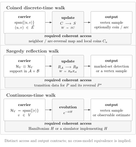
Three quantum-walk models use different state spaces and updates: a coined step $SC$ on directed edges, a Szegedy step $R_{\mathcal B}R_{\mathcal A}$ on coherent transition states, and continuous evolution $e^{-itH}$ on vertices. Their access and readout contracts must be compared separately.

The Ten-Field Quantum-Walk Claim Record

Asymptotic notation compresses a theorem only after its operands have been fixed. The following record instantiates the chapter’s canonical ten fields for element distinctness. Each entry identifies what an algorithm receives, what it must return, and which costs the displayed query bound does and does not contain. A genuinely irrelevant field may be marked N/A only with a reason. An unknown implementation cost remains unknown; an unmeasured hardware quantity remains unmeasured; and a cost deliberately excluded from an oracle model remains excluded from that model. None of those cases is synonymous with not applicable.

Canonical field	Element-distinctness claim
Problem family and size.	An input string $x=(x_0,\ldots,x_{N-1})\in[q]^N$; determine whether two different indices carry the same value.
Promise and instance.	No unique-collision promise is required. A positive instance has at least one pair $i\ne j$ with $x_i=x_j$; a negative instance is injective.
Access and encoding.	Coherent modular-addition value oracle $O_x$, its inverse, and a reversible representation of an $r$-subset with cached values; $2\le r\le N/2$.
Output and use.	Bounded-error decision between a collision and `distinct`; if a pair is requested, it is recovered from the produced marked cache with separately counted reversible work.
Success and error.	Under ideal exact access, constant success with a verifiable marked output and hence one-sided decision error; reducing failure to $\eta$ costs an additional $O(\log(1/\eta))$ repetition factor.
Algorithmic idea.	Search marked vertices of a half-lazy Johnson walk; the marked fraction and the square-root spectral phase gap jointly control the number of coherent updates.
Executable procedure.	Prepare the stationary subset superposition and cache, alternate stationary-state and markedness reflections through the MNRS construction, then verify and read out a marked subset or report no collision.
Resource ledger.	$S=\Theta(r)$, $U=\Theta(1)$, and $C=0$ in value-query units, giving $\Theta(r+N/\sqrt r)=\Theta(N^{2/3})$ at the optimum; gates, coherent memory, controls, inverses, and readout remain separate.
Classical comparator.	Compare with randomized classical algorithms using the same value-oracle input, the same collision promise, a bounded-error decision output, and value-query complexity rather than an explicit-array runtime.
Evidence and limits.	The upper bound is due to Ambainis, with the matching quantum query lower bound established by Aaronson and Shi; neither result alone supplies a fault-tolerant or wall-clock advantage.

The record prevents several common substitutions. An explicit array in random-access memory is not automatically the coherent value oracle used above. A decision algorithm is not automatically a pair-output algorithm. A value-query bound is not an elementary-gate bound, and a matching quantum lower bound does not establish a quantum-versus-classical hardware advantage. Those conversions can be favorable, unfavorable, or unknown, but they must be stated rather than hidden behind the word “walk.”

Discrete-Time Coined Walks

Coin and shift on directed edges

Let $G=(V,E)$ be a finite undirected graph. Its directed-edge, or arc, Hilbert space is

$$\mathcal H_{\rm arc} = \operatorname{span} \{\lvert v,w\rangle:(v,w)\text{ is a directed edge}\}.$$

For each vertex $v$, the outgoing arcs span a local space of dimension $\deg(v)$. A local unitary $C_v$ mixes those outgoing directions, and the global coin is the orthogonal direct sum

$$C=\bigoplus_{v\in V}C_v.$$

The graph-general default here is the flip-flop shift

$$S\lvert v,w\rangle=\lvert w,v\rangle,$$

followed by the frozen step convention

$$W_{\rm coin}=SC.$$

The direct sum is unitary exactly when every $C_v$ is unitary. The shift is a permutation with $S^2=I$, so it is unitary and self-inverse. Thus $W_{\rm coin}$ is unitary. This elementary proof is important operationally: an update that discards a direction label, samples a neighbor, or overwrites a cache is not this coherent walk until it has been embedded in a reversible operation with the necessary workspace.

A common regular-graph choice is the Grover diffusion coin $C_v=2\lvert s_v\rangle\langle s_v\rvert-I$, where $\lvert s_v\rangle$ is uniform over outgoing arcs. It should not be confused with the complete unstructured-search algorithm owned by Grover Search. At a marked vertex one may replace the local coin, apply a separate phase oracle, add a self-loop, or enlarge the coin space. These alternatives can have different spectra and success probabilities. On an irregular graph, padding all local spaces to a common register requires a declared action on unused labels; leaving that action unspecified leaves the purported unitary unspecified.

Order also matters. $SC$ means coin first and route second when operators act from the right, whereas $CS$ routes before mixing. A moving shift preserves a direction label while changing the vertex; a flip-flop shift reverses the directed edge. They may be related on a specially relabeled regular graph, but they are not textually interchangeable. Likewise, measuring after every step produces a classical Markov process, whereas measuring only at a selected time retains multi-step interference. The initial state and sampling rule belong to the walk definition.

Exact interference on a four-cycle

For a compact finite example, use vertices $x\in\mathbb Z_4$ and coin labels $L,R$. This example explicitly changes from the preceding flip-flop default to the named moving shift

$$S\lvert L,x\rangle=\lvert L,x-1\bmod4\rangle, \qquad S\lvert R,x\rangle=\lvert R,x+1\bmod4\rangle.$$

Let the local coin be Hadamard,

$$H\lvert L\rangle =\frac{\lvert L\rangle+\lvert R\rangle}{\sqrt2}, \qquad H\lvert R\rangle =\frac{\lvert L\rangle-\lvert R\rangle}{\sqrt2},$$

define the local coin in the interleaved ordered basis by $C=\bigoplus_{x=0}^{3}H_x$, and set $U=SC$. Starting from $\lvert\psi_0\rangle=\lvert L,0\rangle$, repeated application gives

$$\begin{aligned} \lvert\psi_1\rangle &=\frac{\lvert L,3\rangle+\lvert R,1\rangle}{\sqrt2},\\ \lvert\psi_2\rangle &=\frac{\lvert L,0\rangle+\lvert R,0\rangle +\lvert L,2\rangle-\lvert R,2\rangle}{2},\\ \lvert\psi_3\rangle &=\frac{\lvert L,3\rangle+\lvert R,3\rangle}{\sqrt2},\\ \lvert\psi_4\rangle &=\lvert L,2\rangle. \end{aligned}$$

The cancellations at the third step are visible in the second-step signs. The two amplitudes that could reach vertex $1$ cancel, while the amplitudes at vertex $3$ reinforce. Consequently the coherent position distribution at $t=3$ is concentrated at vertex $3$. A classical simple random walk on the same cycle, begun at vertex $0$, has distribution $(0,1/2,0,1/2)$ after three steps. The difference certifies interference under these conventions. It is not by itself a speedup because no computational problem, access cost, stopping rule, or matched comparator has yet been supplied.

This example also shows why the coin cannot be omitted from a state description. At $t=2$, the position distribution is split evenly between vertices $0$ and $2$, but the conditional coin states carry opposite relative phases. A measurement resolving both position and coin destroys the cross terms needed for the later cancellation. A position-only measurement retains coherence inside each coin subspace and has a different effect. “Measure the walker” is incomplete unless the measured registers and outcome handling are named.

Continuous-Time Quantum Walks

Adjacency and Laplacian generators

A continuous-time walk acts directly on the vertex space. With $\hbar=1$, the adjacency convention used here is

$$U(t)=e^{-itH_{\rm walk}}, \qquad H_{\rm walk}=-\gamma A,$$

where $A$ is the adjacency matrix and $\gamma$ fixes the energy and time scale. The continuous-time computational model introduced by Farhi and Gutmann uses Hamiltonian evolution rather than alternating coin and shift registers. For marked-vertex search, a standard rank-one perturbation is

$$H_{\rm search} =-\gamma A-\lvert w\rangle\langle w\rvert.$$

The initial state, marked vertex $w$, choice of $\gamma$, measurement time, and acceptable time window are all part of the search instance. Rescaling $H$ by $a$ and time by $1/a$ preserves the ideal unitary, so a claim quoting time without a normalization or implementation model is not invariant information.

Some authors use the graph Laplacian $L=D-A$, where $D$ is the degree matrix. On a $k$-regular graph,

$$\gamma L =\gamma kI-\gamma A =\gamma kI+H_{\rm walk},$$

and therefore

$$e^{-it\gamma L} =e^{-i\gamma kt}e^{-itH_{\rm walk}}.$$

The two evolutions have identical measurement probabilities after the sign convention is matched because the extra factor is a global phase. On an irregular graph, $D$ is not proportional to the identity. For the three-vertex path, $D=\operatorname{diag}(1,2,1)$, so the Laplacian adds a vertex-dependent diagonal potential. It changes relative phases and is operationally different from adjacency evolution. “A walk on the same graph” therefore does not determine a continuous-time generator.

Evolution time, measurement, and implementation

Spectral decomposition gives

$$e^{-itH_{\rm walk}} =\sum_j e^{-itE_j}\lvert E_j\rangle\langle E_j\rvert.$$

The moduli of the energy-basis amplitudes are constant, while their phases rotate. In a finite closed system this quasiperiodic behavior generally prevents convergence of the instantaneous vertex distribution. An algorithm may instead choose a specific time, sample a time from an interval, average probabilities over a window, or introduce a measurement or absorbing rule. Each choice defines a different output distribution. Hitting time, detection time, and time to produce a marked vertex should not be used as synonyms unless a theorem proves their equivalence in the stated model.

The two-vertex graph makes the time scale explicit. Its adjacency is the Pauli matrix $X$, so $H=-\gamma X$ and

$$e^{-itH} =e^{i\gamma tX} =\cos(\gamma t)I+i\sin(\gamma t)X.$$

From $\lvert0\rangle$, the state is $\cos(\gamma t)\lvert0\rangle+i\sin(\gamma t)\lvert1\rangle$, and the transition probability is $\sin^2(\gamma t)$. Perfect transfer first occurs at $t=\pi/(2\gamma)$. That value is an ideal evolution time, not a gate count.

An executable claim must state how the Hamiltonian is supplied, bound $\lVert H\rVert$, allocate simulation error, prepare the initial state, implement the marked potential, and measure the result. If the Hamiltonian is a physical interaction, calibration, control, and readout remain costs. If it is simulated by a circuit, oracle normalization, queries, gates, ancillas, and precision must be expanded through Hamiltonian Simulation Algorithms. The exact conversion between continuous and discrete walks developed by Childs is a mathematical construction with explicit overhead, not permission to call physical time a circuit depth.

Reversible Markov Chains and Szegedy Quantization

Time reversal, transition subspaces, and discriminant

Let $P=(p_{xy})$ be a finite irreducible row-stochastic Markov chain, so $p_{xy}$ is the probability of moving from $x$ to $y$. Let $\pi$ be stationary, $\pi^{\mathsf T}P=\pi^{\mathsf T}$, and define the time-reversed transition matrix by

$$\pi_xp_{xy}=\pi_yp^*_{yx}.$$

The coherent outgoing and reversed states are

$$\lvert p_x\rangle =\sum_y\sqrt{p_{xy}}\lvert y\rangle, \qquad \lvert p_y^*\rangle =\sum_x\sqrt{p^*_{yx}}\lvert x\rangle.$$

They define two subspaces of the doubled state space,

$$\mathcal A =\operatorname{span}\{\lvert x\rangle\lvert p_x\rangle\}, \qquad \mathcal B =\operatorname{span}\{\lvert p_y^*\rangle\lvert y\rangle\}.$$

With $R_{\mathcal A}=2\Pi_{\mathcal A}-I$ and $R_{\mathcal B}=2\Pi_{\mathcal B}-I$, the convention throughout this page is

$$W(P)=R_{\mathcal B}R_{\mathcal A}.$$

Operationally, reflecting about $\mathcal A$ requires coherently preparing and unpreparing each transition state $\lvert p_x\rangle$; reflecting about $\mathcal B$ requires the corresponding time-reversed access. Reversibility can simplify these circuits, but the abstract identity $P=P^*$ does not itself synthesize them. Registers storing transition data, controls, inverse calls, and numerical probabilities belong to the access contract.

The overlap between the two subspaces is encoded by the discriminant

$$D(P)_{xy}=\sqrt{p_{xy}p^*_{yx}}.$$

When detailed balance holds, $P=P^*$ and

$$D(P) =\operatorname{diag}(\pi)^{1/2} P\operatorname{diag}(\pi)^{-1/2}$$

is symmetric and similar to $P$. Thus it has the same real eigenvalues, while its singular values are their absolute values. The coherent stationary state

$$\lvert\Pi\rangle =\sum_x\sqrt{\pi_x}\lvert x\rangle\lvert p_x\rangle$$

lies in the common stationary sector. Szegedy’s quantization turns these overlaps into eigenphases of a product of reflections.

From singular values to walk phases

Suppose a nontrivial singular value is $\sigma_j(D)=\cos\theta_j$ with $0<\sigma_j<1$. The associated principal two-dimensional subspace is invariant under both reflections. Their product is a rotation through twice the principal angle, so under the frozen order $R_{\mathcal B}R_{\mathcal A}$ the walk eigenvalues are

$$e^{\pm2i\theta_j}.$$

Changing the reflection order conjugates these phases. The singular sectors at $1$ and $0$ require separate treatment. At singular value $1$, the subspaces intersect and include a zero-phase stationary direction. At singular value $0$, the principal angle is $\pi/2$ and the product acts in a degenerate phase-$\pi$ sector; forcing the generic paired notation onto either endpoint obscures multiplicities and invariant complements.

For a lazy reversible chain, define the absolute spectral gap

$$\delta =1-\max_{\lambda\ne1}\lvert\lambda(P)\rvert.$$

Laziness excludes a nearly bipartite eigenvalue near $-1$ from masquerading as rapid mixing. The smallest relevant nonzero walk phase satisfies

$$\Delta =2\arccos(1-\delta) \ge2\sqrt\delta, \qquad \Delta=\Theta(\sqrt\delta)$$

as $\delta\to0$. The square root is the spectral source of the walk-search improvement. It is not a statement that every classical hitting time is square-rooted: the marked overlap, setup, update, check, and output procedure still enter.

For a nonreversible chain, the discriminant need not be similar to $P$ as a symmetric matrix. A valid extension can be formulated using a singular-value gap of the appropriate discriminant or a related reversible construction. Substituting an ordinary eigenvalue gap into the reversible theorem without proving the necessary spectral relationship is not justified. Even in the reversible case, a stated “gap” must say whether it is $1-\lambda_2$, an absolute gap, a singular-value gap, or the induced phase gap.

Search by Quantum Walk

Detection, finding, and the stationary reflection

Let $M$ be a marked subset of the Markov-chain state space. A coherent check may act as a phase oracle, multiplying $\lvert x\rangle$ by $-1$ exactly when $x\in M$, while preserving maintained data. Detection asks whether $M$ is empty. Finding asks for a classical marked state, and coherent production asks for a state supported substantially on $M$. Finding can imply detection after verification, but a detection routine that only produces a bit need not reveal a witness. A hitting-time statement must identify which task it solves.

For an ergodic chain, the stationary state is the distinguished zero-phase direction in the relevant invariant subspace contained in $\mathcal A+\mathcal B$. That restriction matters: $\mathcal A^\perp\cap\mathcal B^\perp$ can contribute an additional $+1$ sector to the full product of reflections, so phase zero on the entire doubled Hilbert space does not by itself identify the stationary vector. The algorithm prepares and remains in the transition-generated invariant subspace. There an ideal stationary reflection preserves the stationary component and reverses the orthogonal components. Phase estimation can approximate this restricted operation by resolving phase zero from phases whose magnitudes are at least $\Delta$. The required phase resolution is therefore proportional to

$$\frac1\Delta=O\!\left(\frac1{\sqrt\delta}\right).$$

This argument explains the gap dependence but does not make phase estimation free. It requires controlled powers or controlled walk steps, inverse uncomputation, a resolution and failure budget, and clean phase workspace. The powered-unitary construction belongs to Quantum Phase Estimation. Likewise, arranging repeated reflections to rotate amplitude toward marked space belongs to Amplitude Amplification; the walk theorem below instantiates rather than rederives that machinery. The log-free MNRS theorem must not be reconstructed by repeating one fixed-precision approximate reflection: its robust variable-precision construction is what avoids that naive extra logarithm.

Under ideal exact markedness verification, one can use a one-sided decision convention: a returned witness is checked, so a negative instance never produces a false verified collision, while a positive instance may be missed with bounded probability. Approximate transitions and checks can spoil that property unless their errors are incorporated into the decision rule. “Bounded error” must therefore name which side can err and whether the claim concerns an ideal oracle algorithm or its approximate implementation.

The MNRS setup–update–check theorem

Let $P$ be a finite reversible ergodic chain. When $M\ne\varnothing$, suppose its stationary measure obeys $\pi(M)\ge\epsilon>0$, and let $\delta$ be the absolute spectral gap. The Magniez–Nayak–Roland–Santha framework assigns three costs:

• $S$ prepares the coherent stationary state together with all maintained data;
• $U$ implements coherent $P$ and $P^*$ transitions, including the inverses actually required by the walk; and
• $C$ implements a markedness phase check using the maintained data.

The bounded-error cost is

$$O\!\left[ S+ \frac1{\sqrt\epsilon} \left( \frac{U}{\sqrt\delta}+C \right) \right].$$

This theorem, proved in Search via Quantum Walk, has a universal constant success probability under its hypotheses. Repeating an independently verifiable procedure reduces failure to $\eta$ with a normally sufficient $O(\log(1/\eta))$ multiplicative factor. A more specialized amplification schedule may improve constants, but it must retain its own access and error conditions.

The formula is a typed cost expression, not a count of anonymous elementary operations. If $S,U,C$ are measured in value-oracle queries, the conclusion is in value-oracle queries. If each is a vector containing queries, gates, depth, and memory traffic, the expression can be evaluated componentwise only where the same coherent construction supports those currencies. Controlled transitions, inverse operations, phase resolution, clean work registers, and coherent data access remain implementation obligations. They cannot be inferred from a classical routine that samples one step of $P$.

The theorem should also state its output. For detection, the algorithm distinguishes $M=\varnothing$ from stationary marked weight at least $\epsilon$. For finding, it must produce and verify a marked state, potentially adding readout or repetition. If the maintained data already contains a witness, the check and witness extraction may use no further input queries while still consuming reversible gates. That distinction is central in element distinctness.

Element Distinctness on the Johnson Graph

Marked fraction and the lazy Johnson gap

Let the input be $x\in[q]^N$, supplied by the coherent value oracle

$$O_x\lvert i,a,z\rangle = \lvert i,(a+x_i)\bmod q,z\rangle.$$

The extra register $z$ denotes maintained workspace left unchanged by this query. The decision output is either that a collision exists or `distinct`; producing indices requires the marked subset’s cache to be inspected reversibly and then measured. Ambainis’s algorithm stores an $r$-subset $R\subset[N]$ and the associated values $\{x_i:i\in R\}$. A subset is marked if its cache contains two equal values.

Use the Johnson graph $J(N,r)$, whose vertices are $r$-subsets and whose edges exchange one selected index with one unselected index. The swap chain has degree $r(N-r)$ and the uniform stationary distribution. To freeze the absolute-gap convention and avoid negative-spectrum complications, use the half-lazy transition

$$P=\frac12(I+P_{\rm swap}), \qquad 2\le r\le\frac N2.$$

If the input contains a fixed colliding pair, the fraction of subsets containing both indices is

$$\epsilon =\frac{\binom{N-2}{r-2}}{\binom Nr} =\frac{r(r-1)}{N(N-1)}.$$

Additional collision pairs can only increase the marked fraction, so this is a valid lower bound without a unique-collision promise. The adjacency eigenvalues of the swap graph are

$$\theta_j =(r-j)(N-r-j)-j =r(N-r)-j(N-j+1).$$

After normalization by the degree and half-lazification, the eigenvalues become

$$\mu_j =1- \frac{j(N-j+1)}{2r(N-r)}.$$

The first nonstationary value is $\mu_1=1-N/[2r(N-r)]$. In the stated range, the lazy spectrum is nonnegative and no lower eigenvalue has larger absolute value, so

$$\delta =\frac{N}{2r(N-r)}.$$

These exact combinatorial and spectral identities are the bridge from the chosen data structure to the MNRS theorem. Replacing the Johnson walk by a different subset update changes the gap and must be reaudited.

Optimizing subset size and query cost

Preparing the stationary cache queries $r$ values, so $S=\Theta(r)$. A coherent exchange updates only constantly many cached values, giving $U=\Theta(1)$ value-query cost under the standard cached-update convention. Once values are stored, detecting a duplicate uses $C=0$ additional value queries, although comparison networks, routing, flags, and their inverses still use gates and workspace. Substitution gives

$$\begin{aligned} S+\frac{U}{\sqrt{\epsilon\delta}} &=\Theta\!\left( r+ \sqrt{\frac{2(N-1)(N-r)}{r-1}} \right)\\ &=\Theta\!\left(r+\frac N{\sqrt r}\right). \end{aligned}$$

Balancing $r$ with $N/\sqrt r$ gives $r=\Theta(N^{2/3})$ and total bounded-error value-query complexity $\Theta(N^{2/3})$. The construction is due to Ambainis. The lower bound of Aaronson and Shi shows that this scaling is optimal in the corresponding quantum query model. Optimal query scaling does not imply that the cached data structure, coherent comparisons, or fault-tolerant implementation is optimal.

For the finite substitution $N=64$, $r=16$,

$$\epsilon=\frac5{84}, \qquad \delta=\frac1{24}, \qquad \Delta=2\arccos\frac{23}{24},$$

and

$$\frac1{\sqrt{\epsilon\delta}} =12\sqrt{\frac{14}{5}}, \qquad 16+12\sqrt{\frac{14}{5}} \approx36.0798406368.$$

The last number is a finite parameter substitution inside an asymptotic cost theorem under a unit-cost update convention. It is not an exact integer query count. If a reversible cache replacement is priced at two oracle calls, the same substitution becomes

$$16+24\sqrt{\frac{14}{5}} \approx56.1596812736.$$

The exponent is unchanged, but the ledger is honest about the convention. Storing $r$ indices and $r$ values already needs at least

$$r\bigl(\lceil\log_2N\rceil+\lceil\log_2q\rceil\bigr)$$

logical data qubits in a straightforward representation, before subset-ordering data, the walk coin, collision flags, routing workspace, and error correction. Reporting the query theorem without this memory boundary would misdescribe what must be executed.

Spatial Search and Oracle Traversal Are Model-Dependent

Spatial-search results depend sharply on graph dimension, degree, boundary conditions, locality, marked multiplicity, marking geometry, coin choice, self-loops, initial state, access, and whether the task is detection or finding. The search Hamiltonian $-\gamma A-\lvert w\rangle\langle w\rvert$ does not have the same avoided crossing or marked-state overlap on every graph. Childs and Goldstone found $O(\sqrt N)$ continuous-time search with constant-order success for their periodic-lattice construction when $d>4$. At the critical dimension $d=4$, the fixed-Hamiltonian evolution lasts $\Theta(\sqrt{N\log N})$ but reaches the mark with only $\Theta(1/\log N)$ probability. Independent verified repetition therefore costs $O(\sqrt N\log^{3/2}N)$, while amplitude amplification can give $O(\sqrt N\log N)$ only when the required reflection and inverse access are licensed. For $d<4$, that construction gives no substantial speedup. These are not generic bounds for graphs of order $N$.

Discrete coined search has equally specific hypotheses. Shenvi, Kempe, and Whaley analyzed a unique marked item on the hypercube with a particular coin and symmetry reduction. For a two-dimensional grid with one marked vertex, Ambainis, Kempe, and Rivosh obtained $O(\sqrt N\log N)$ steps under their coined-walk conventions. Tulsi’s ancilla-controlled modification improves the two-dimensional scaling to $O(\sqrt{N\log N})$. The logarithm, ancilla, start state, marked multiplicity, boundary conditions, and readout procedure cannot be dropped when transplanting either result to another lattice.

Traversal gives a different lesson. Childs, Cleve, Deotto, Farhi, Gutmann, and Spielman constructed a continuous-time walk that traverses an implicitly supplied glued-tree graph with an exponential oracle separation from classical algorithms in that problem. The instance is not an arbitrary explicit graph: its layered structure is promised while vertex labels are hidden behind an adjacency oracle. The output is the exit label reached from the entrance. The result is therefore evidence that coherent propagation can exploit a specially promised oracle graph, not a theorem of generic exponential advantage for graph search, shortest paths, or explicit adjacency lists.

The safe reporting pattern is model first, bound second. State whether the graph is explicit or oracle supplied; whether degree and geometry are promised; how neighbors, marks, and edge weights are queried; how the initial state is prepared; which walk model is used; how long it runs and when it is measured; what counts as success; and what the classical comparator receives. Only then can a polynomial or exponential separation be interpreted. Ballistic spreading of an unmarked wave packet supplies none of those problem-level fields by itself.

From Walk Queries to Executable Resources

Approximation errors accumulate through the actual sequence. If ideal and implemented discrete steps obey $\lVert\widetilde W-W\rVert\le\varepsilon_{\rm step}$, telescoping gives

$$\begin{aligned} \widetilde W^T-W^T &=\sum_{j=0}^{T-1} \widetilde W^{T-1-j}(\widetilde W-W)W^j,\\ \lVert\widetilde W^T-W^T\rVert &\le T\lVert\widetilde W-W\rVert \le T\varepsilon_{\rm step}. \end{aligned}$$

For normalized initial states, the final state-vector difference is at most $T\varepsilon_{\rm step}$. If $\Pi_M$ is the declared success projector, expanding the difference of quadratic forms gives the conservative probability bound

$$\left| \langle\widetilde\psi\rvert\Pi_M\lvert\widetilde\psi\rangle -\langle\psi\rvert\Pi_M\lvert\psi\rangle \right| \le2T\varepsilon_{\rm step}.$$

This worst-case linear estimate may be loose, but replacing it by an assumed incoherent square-root law would be unjustified. Stationary-state preparation error, transition-state preparation error, inverse mismatch, marked-check error, phase-resolution error, and final sampling error should remain separate ledger entries until a proved composition rule combines them.

Continuous-time implementations have their own budgets. For Hermitian $H$ and $\widetilde H$ under a common time convention, a Duhamel estimate gives

$$\lVert e^{-it\widetilde H}-e^{-itH}\rVert \le |t|\lVert\widetilde H-H\rVert.$$

A simulation algorithm then adds approximation and synthesis error beyond any modeling error in the generator. The norm, time, target precision, oracle normalization, and failure probability all influence circuit resources. Physical evolution for time $t$ and a digital approximation of $e^{-itH}$ are different resource statements even when their ideal unitaries coincide.

A complete ledger distinguishes input-oracle queries; controlled and inverse queries; coherent random-access operations; elementary gates and non-Clifford gates; depth; clean and dirty ancillas; cached indices and values; stationary or initial-state preparation; walk steps; physical evolution time; measurements; repetitions; and classical postprocessing. It also records which cost is worst-case, expected, or amortized. A zero query check may have a large reversible-gate cost, and a constant-degree graph update may still require expensive address translation.

Failure reduction is not hidden in “bounded error.” If one independent verified trial succeeds with probability at least a constant $p_0>0$, then $k$ failures have probability at most $(1-p_0)^k$, so $k=O(\log(1/\eta))$ suffices for failure at most $\eta$. Coherent amplification can have a different dependence, but it requires the licensed reflections and inverses specified by its owner. Sampling an unverified bit and taking a majority may be two-sided rather than one-sided. The chosen procedure belongs in the claim.

Finally, a matched comparator receives the same input representation, promise, output information, and error criterion. Comparing a quantum neighbor oracle with a classical explicit adjacency matrix, or a quantum decision bit with a classical list of all collisions, does not isolate the walk’s contribution. Query Complexity supplies the general discipline for these comparisons; the present page specializes it to walk access and outputs.

Relationships, Boundaries, and Matched Comparisons

Quantum walks assemble reusable ingredients but do not take ownership of them. Algorithmic Primitives supplies the access–transform–readout vocabulary used to organize each procedure. Grover Search remains the canonical home of the exact two-dimensional unstructured-search rotation, while Amplitude Amplification owns general reflection schedules and failure management. Quantum Phase Estimation owns eigenphase readout; this page uses only its restricted stationary-reflection consequence.

Quantum Algorithms for Optimization specializes walk and search-tree primitives to optimization route selection and matched output-resource comparisons; this page retains the walk models, access contracts, and spectral search guarantees.

Quantum Oracles owns full-space interface semantics and licenses controlled or inverse access. Block Encodings and QSVT may encode and transform a walk operator, but it does not own graph hitting or search guarantees. Qubitization and Quantum Signal Processing owns the specialized Hamiltonian signal-walk and phase-synthesis workflow; that signal walk is not the generic coined or Szegedy model. Hamiltonian Simulation Algorithms owns the expansion from a continuous-time generator to simulation queries and gates.

The classical analogy should remain typed. A classical transition matrix evolves probabilities and may mix; a Szegedy walk coherently encodes transition amplitudes and remains unitary. Classical mixing parameters help determine the quantum phase gap, but the quantum procedure still needs coherent transition preparation and a marked reflection. Conversely, a fast classical sampler for $P$ need not give a comparably fast coherent preparation circuit. The page therefore excludes experimental transport, decoherence, topological phases, universal computation by walks, a general Markov-chain textbook, and extended optimization case studies. Those subjects require different canonical homes and evidence.

Three Reproducible Finite Audits

Finite examples cannot prove an asymptotic theorem, but they can expose convention, phase, normalization, and table errors. The three audits below are small enough for exact hand calculation and are reproduced by one dependency-free program at tolerance $10^{-12}$.

Audit 1 — Coined evolution on C₄

Use the ordered basis $(\lvert L,0\rangle,\lvert R,0\rangle,\ldots,\lvert L,3\rangle,\lvert R,3\rangle)$, the explicitly named moving shift from the four-cycle example, the local direct-sum coin $C=\bigoplus_{x=0}^{3}H_x$, the step $U=SC$, and $\lvert\psi_0\rangle=\lvert L,0\rangle$. Direct matrix checks give $C^\dagger C=S^\dagger S=U^\dagger U=I_8$. Every listed state has norm one.

$t$	exact state	$(p_0,p_1,p_2,p_3)$
$0$	$\lvert L,0\rangle$	$(1,0,0,0)$
$1$	$(\lvert L,3\rangle+\lvert R,1\rangle)/\sqrt2$	$(0,1/2,0,1/2)$
$2$	$(\lvert L,0\rangle+\lvert R,0\rangle+\lvert L,2\rangle-\lvert R,2\rangle)/2$	$(1/2,0,1/2,0)$
$3$	$(\lvert L,3\rangle+\lvert R,3\rangle)/\sqrt2$	$(0,0,0,1)$
$4$	$\lvert L,2\rangle$	$(0,0,1,0)$

Audit 2 — A two-state Szegedy walk

Consider

$$P= \begin{pmatrix} 3/4&1/4\\ 1/2&1/2 \end{pmatrix}.$$

The stationary distribution is $\pi=(2/3,1/3)$, and detailed balance makes the chain reversible. Its discriminant is

$$D= \begin{pmatrix} 3/4&1/(2\sqrt2)\\ 1/(2\sqrt2)&1/2 \end{pmatrix}.$$

It is positive symmetric with singular values $1$ and $1/4$. The nonstationary eigenvalue of $P$ is $1/4$, so the absolute gap is $3/4$, and the frozen reflection order predicts phases $\pm2\arccos(1/4)$.

The executable audit also constructs the two transition isometries and both reflections rather than inferring the walk spectrum from $D$ alone. For the ordered doubled basis $(\lvert00\rangle,\lvert01\rangle,\lvert10\rangle,\lvert11\rangle)$, it verifies

$$\chi_W(z) = \frac{(z-1)^2(4z^2+7z+4)}4.$$

Thus $W$ has the predicted conjugate pair and two $+1$ eigenvalues: the coherent stationary vector in $\mathcal A\cap\mathcal B$ and one vector in $\mathcal A^\perp\cap\mathcal B^\perp$. This finite example makes the invariant-subspace restriction in the search construction concrete.

quantity	exact prediction	computed result
stationary distribution	$\pi=(2/3,1/3)$	$(0.666666666666667,0.333333333333333)$
stationarity	$\pi^{\mathsf T}P=\pi^{\mathsf T}$	maximum residual $0$
detailed balance	$\pi_0p_{01}=\pi_1p_{10}=1/6$	both sides $0.166666666666667$
discriminant	$D_{00}=3/4$, $D_{01}=D_{10}=1/(2\sqrt2)$, $D_{11}=1/2$	entries $(0.75,0.353553390593274,0.353553390593274,0.5)$
discriminant symmetry	$D=D^{\mathsf T}$	maximum antisymmetric residual $0$
singular values	$(1,1/4)$	$(1,0.25)$
absolute gap	$1-\lvert1/4\rvert=3/4$	$0.75$
paired walk phases	$\pm2\arccos(1/4)$	$\pm2.636232143305636$

Audit 3 — Two-vertex continuous evolution

Set $H=-\gamma X$ and begin in $\lvert0\rangle$. Since $X^2=I$,

$$e^{i\gamma tX} =\cos(\gamma t)I+i\sin(\gamma t)X,$$

so the norm is one and $p_{0\to1}(t)=\sin^2(\gamma t)$. The selected times cover the first quarter-period from the initial vertex to perfect transfer.

$t$	$p_0(t)$	$p_1(t)$
$0$	$1$	$0$
$\pi/(8\gamma)$	$(2+\sqrt2)/4$	$(2-\sqrt2)/4$
$\pi/(4\gamma)$	$1/2$	$1/2$
$3\pi/(8\gamma)$	$(2-\sqrt2)/4$	$(2+\sqrt2)/4$
$\pi/(2\gamma)$	$0$	$1$

const tolerance = 1e-12;

function close(actual, expected, label) {
  if (Math.abs(actual - expected) > tolerance) {
    throw new Error(label + ': ' + actual + ' != ' + expected);
  }
}

function multiply(a, b) {
  return a.map((row) =>
    b[0].map((_, j) =>
      row.reduce((sum, value, k) => sum + value * b[k][j], 0),
    ),
  );
}

function transpose(a) {
  return a[0].map((_, j) => a.map((row) => row[j]));
}

function identity(n) {
  return Array.from({ length: n }, (_, i) =>
    Array.from({ length: n }, (_, j) => (i === j ? 1 : 0)),
  );
}

function checkOrthogonal(a, label) {
  const product = multiply(transpose(a), a);
  const size = product.length;
  const target = identity(size);
  for (let i = 0; i < size; i += 1) {
    for (let j = 0; j < size; j += 1) {
      close(product[i][j], target[i][j], label + '[' + i + ',' + j + ']');
    }
  }
}

const dimension = 8;
const coin = Array.from({ length: dimension }, () => Array(dimension).fill(0));
for (let x = 0; x < 4; x += 1) {
  coin[2 * x][2 * x] = 1 / Math.sqrt(2);
  coin[2 * x][2 * x + 1] = 1 / Math.sqrt(2);
  coin[2 * x + 1][2 * x] = 1 / Math.sqrt(2);
  coin[2 * x + 1][2 * x + 1] = -1 / Math.sqrt(2);
}

const shift = Array.from({ length: dimension }, () => Array(dimension).fill(0));
for (let x = 0; x < 4; x += 1) {
  shift[2 * ((x + 3) % 4)][2 * x] = 1;
  shift[2 * ((x + 1) % 4) + 1][2 * x + 1] = 1;
}

const step = multiply(shift, coin);
checkOrthogonal(coin, 'coin unitarity');
checkOrthogonal(shift, 'shift unitarity');
checkOrthogonal(step, 'step unitarity');

function apply(matrix, vector) {
  return matrix.map((row) =>
    row.reduce((sum, value, j) => sum + value * vector[j], 0),
  );
}

const expectedPositions = [
  [1, 0, 0, 0],
  [0, 0.5, 0, 0.5],
  [0.5, 0, 0.5, 0],
  [0, 0, 0, 1],
  [0, 0, 1, 0],
];
const expectedAmplitudes = [
  [1, 0, 0, 0, 0, 0, 0, 0],
  [0, 0, 0, 1 / Math.sqrt(2), 0, 0, 1 / Math.sqrt(2), 0],
  [1 / 2, 1 / 2, 0, 0, 1 / 2, -1 / 2, 0, 0],
  [0, 0, 0, 0, 0, 0, 1 / Math.sqrt(2), 1 / Math.sqrt(2)],
  [0, 0, 0, 0, 1, 0, 0, 0],
];

let state = Array(dimension).fill(0);
state[0] = 1;
for (let t = 0; t < expectedPositions.length; t += 1) {
  for (let k = 0; k < dimension; k += 1) {
    close(state[k], expectedAmplitudes[t][k], 'C4 amplitude t=' + t + ' k=' + k);
  }
  const probabilities = Array(4).fill(0);
  for (let x = 0; x < 4; x += 1) {
    probabilities[x] = state[2 * x] ** 2 + state[2 * x + 1] ** 2;
    close(probabilities[x], expectedPositions[t][x], 'C4 t=' + t + ' x=' + x);
  }
  close(
    probabilities.reduce((sum, value) => sum + value, 0),
    1,
    'C4 norm t=' + t,
  );
  state = apply(step, state);
}

const transition = [
  [3 / 4, 1 / 4],
  [1 / 2, 1 / 2],
];
const stationary = [2 / 3, 1 / 3];
for (let y = 0; y < 2; y += 1) {
  const evolved = stationary.reduce(
    (sum, value, x) => sum + value * transition[x][y],
    0,
  );
  close(evolved, stationary[y], 'stationarity ' + y);
}
close(
  stationary[0] * transition[0][1],
  stationary[1] * transition[1][0],
  'detailed balance',
);

const reversed = Array.from({ length: 2 }, (_, y) =>
  Array.from(
    { length: 2 },
    (_, x) => stationary[x] * transition[x][y] / stationary[y],
  ),
);
const discriminantFromProbabilities = Array.from({ length: 2 }, (_, x) =>
  Array.from(
    { length: 2 },
    (_, y) => Math.sqrt(transition[x][y] * reversed[y][x]),
  ),
);
const aIsometry = [
  [Math.sqrt(3) / 2, 0],
  [1 / 2, 0],
  [0, 1 / Math.sqrt(2)],
  [0, 1 / Math.sqrt(2)],
];
const bIsometry = [
  [Math.sqrt(3) / 2, 0],
  [0, 1 / Math.sqrt(2)],
  [1 / 2, 0],
  [0, 1 / Math.sqrt(2)],
];
checkOrthogonal(aIsometry, 'A isometry');
checkOrthogonal(bIsometry, 'B isometry');
const discriminant = multiply(transpose(aIsometry), bIsometry);
for (let x = 0; x < 2; x += 1) {
  for (let y = 0; y < 2; y += 1) {
    close(
      discriminant[x][y],
      discriminantFromProbabilities[x][y],
      'discriminant overlap [' + x + ',' + y + ']',
    );
  }
}
close(discriminant[0][0], 3 / 4, 'D00');
close(discriminant[0][1], 1 / (2 * Math.sqrt(2)), 'D01');
close(discriminant[1][0], discriminant[0][1], 'D symmetry');
close(discriminant[1][1], 1 / 2, 'D11');

function eigenvaluesSymmetric2(a) {
  const trace = a[0][0] + a[1][1];
  const radius = Math.sqrt(
    ((a[0][0] - a[1][1]) / 2) ** 2 + a[0][1] ** 2,
  );
  return [trace / 2 + radius, trace / 2 - radius];
}

const gram = multiply(transpose(discriminant), discriminant);
const singularValues = eigenvaluesSymmetric2(gram)
  .map((value) => Math.sqrt(Math.max(0, value)))
  .sort((a, b) => b - a);
close(singularValues[0], 1, 'largest singular value');
close(singularValues[1], 1 / 4, 'second singular value');

function reflectionFromIsometry(isometry) {
  const projector = multiply(isometry, transpose(isometry));
  return projector.map((row, i) =>
    row.map((value, j) => 2 * value - (i === j ? 1 : 0)),
  );
}

function trace(matrix) {
  return matrix.reduce((sum, row, i) => sum + row[i], 0);
}

function determinant(matrix) {
  const work = matrix.map((row) => row.slice());
  let sign = 1;
  let value = 1;
  for (let column = 0; column < work.length; column += 1) {
    let pivot = column;
    for (let row = column + 1; row < work.length; row += 1) {
      if (Math.abs(work[row][column]) > Math.abs(work[pivot][column])) {
        pivot = row;
      }
    }
    if (Math.abs(work[pivot][column]) < tolerance) return 0;
    if (pivot !== column) {
      [work[pivot], work[column]] = [work[column], work[pivot]];
      sign *= -1;
    }
    const diagonal = work[column][column];
    value *= diagonal;
    for (let row = column + 1; row < work.length; row += 1) {
      const factor = work[row][column] / diagonal;
      for (let k = column + 1; k < work.length; k += 1) {
        work[row][k] -= factor * work[column][k];
      }
    }
  }
  return sign * value;
}

const reflectionA = reflectionFromIsometry(aIsometry);
const reflectionB = reflectionFromIsometry(bIsometry);
const szegedyWalk = multiply(reflectionB, reflectionA);
checkOrthogonal(reflectionA, 'reflection A unitarity');
checkOrthogonal(reflectionB, 'reflection B unitarity');
checkOrthogonal(szegedyWalk, 'Szegedy walk unitarity');

const stationaryWalkState = [
  1 / Math.sqrt(2),
  1 / Math.sqrt(6),
  1 / Math.sqrt(6),
  1 / Math.sqrt(6),
];
const ambientPlusOneState = [
  1 / Math.sqrt(10),
  -Math.sqrt(3 / 10),
  -Math.sqrt(3 / 10),
  Math.sqrt(3 / 10),
];
for (const [label, vector] of [
  ['stationary +1 vector', stationaryWalkState],
  ['ambient +1 vector', ambientPlusOneState],
]) {
  const evolved = apply(szegedyWalk, vector);
  for (let k = 0; k < vector.length; k += 1) {
    close(evolved[k], vector[k], label + ' k=' + k);
  }
}

close(trace(szegedyWalk), 1 / 4, 'Szegedy walk trace');
close(trace(multiply(szegedyWalk, szegedyWalk)), 49 / 16, 'Szegedy walk square trace');
for (const z of [-2, -1, 0, 1, 2]) {
  const characteristicMatrix = szegedyWalk.map((row, i) =>
    row.map((entry, j) => (i === j ? z : 0) - entry),
  );
  const expectedCharacteristic = ((z - 1) ** 2 * (4 * z ** 2 + 7 * z + 4)) / 4;
  close(
    determinant(characteristicMatrix),
    expectedCharacteristic,
    'Szegedy characteristic polynomial z=' + z,
  );
}

const transitionEigenvalues = [
  1,
  transition[0][0] + transition[1][1] - 1,
];
const absoluteGap =
  1 - Math.max(...transitionEigenvalues.slice(1).map(Math.abs));
close(absoluteGap, 3 / 4, 'absolute gap');
close(
  2 * Math.acos(singularValues[1]),
  2.636232143305636,
  'paired phase magnitude',
);
close(
  Math.acos((trace(szegedyWalk) - 2) / 2),
  2 * Math.acos(singularValues[1]),
  'walk-spectrum phase magnitude',
);

const gamma = 1;
const times = [0, Math.PI / 8, Math.PI / 4, 3 * Math.PI / 8, Math.PI / 2];
const expectedContinuous = [
  [1, 0],
  [(2 + Math.sqrt(2)) / 4, (2 - Math.sqrt(2)) / 4],
  [1 / 2, 1 / 2],
  [(2 - Math.sqrt(2)) / 4, (2 + Math.sqrt(2)) / 4],
  [0, 1],
];

for (let j = 0; j < times.length; j += 1) {
  const angle = gamma * times[j];
  const amplitude0 = Math.cos(angle);
  const imaginaryAmplitude1 = Math.sin(angle);
  const probability0 = amplitude0 ** 2;
  const probability1 = imaginaryAmplitude1 ** 2;
  close(probability0, expectedContinuous[j][0], 'CT p0 row=' + j);
  close(probability1, expectedContinuous[j][1], 'CT p1 row=' + j);
  close(probability0 + probability1, 1, 'CT norm row=' + j);
}

console.log('Quantum-walk-algorithms audits: PASS');

Common Quantum-Walk Claim Failures

“Quantum walks are always quadratically faster.” There is no such theorem. The MNRS expression contains both the marked fraction and a chain-specific spectral gap, while spatial results depend on geometry, marking, and readout. Some problems have polynomial improvements, some oracle separations are exponential, and some walk constructions have no useful advantage.

Ballistic spreading as sufficient evidence of an algorithmic speedup. A position variance can grow faster for a coherent walk than for a classical random walk, but variance is not a computational output. A speedup requires a problem, matched access, a success criterion, and total cost. The four-cycle audit demonstrates interference only.

A graph-size bound without an access model or bit-input parameter. The same $N$-vertex graph may be supplied explicitly, through neighbor queries, by a succinct circuit, or as a physical coupling network. These representations can differ exponentially in input length and loading cost, so a bare dependence on $N$ is ambiguous.

A hitting-time claim that does not distinguish detection from finding. Detecting nonempty marked space, sampling a marked vertex, and outputting a verified witness need different readout and repetition steps. State the output and whether the bound is worst-case, expected, or a randomly sampled observation time.

Physical evolution time $t$ reported as a circuit or query count. Ideal $e^{-itH}$ specifies dynamics. Circuit resources also depend on the Hamiltonian interface, norm, simulation algorithm, error, controls, and synthesis. Physical implementations add calibration and measurement costs rather than eliminating them.

Generic $O(\sqrt N)$ spatial search. Complete graphs, hypercubes, lattices of different dimensions, and irregular graphs have different spectra and marked-state overlaps. Every spatial bound retains its graph family, dimension, boundary conditions, coin or generator, start state, and marking promise.

Generic exponential quantum-walk advantage. The glued-tree separation is an oracle result for a promised implicitly labeled traversal problem. It cannot be promoted to arbitrary graph search, explicit-graph runtime, or practical advantage without new reductions and resource evidence.

Exercises

1. Unitarity of a coined step. Let $C=\bigoplus_v C_v$ with every $C_v$ unitary, and let $S\lvert v,w\rangle=\lvert w,v\rangle$. Prove that $C$, $S$, and $SC$ are unitary. Identify what fails if a proposed “shift” erases the incoming vertex label.

Solution

The arc space is an orthogonal direct sum of the outgoing subspaces at each vertex. Therefore

$$C^\dagger C =\bigoplus_v C_v^\dagger C_v =\bigoplus_v I_v =I_{\rm arc}.$$

The shift permutes the directed-edge basis and satisfies $S^2=I$, hence $S^{-1}=S=S^\dagger$. It follows that

$$(SC)^\dagger(SC) =C^\dagger S^\dagger SC =C^\dagger C =I_{\rm arc}.$$

If a map sends $\lvert v,w\rangle$ only to $\lvert w\rangle$, then distinct incoming arcs can acquire the same output. The map is not injective, does not preserve inner products, and cannot be a unitary shift. A reversible implementation must retain enough direction or workspace information to reconstruct the input.

2. Measurement inside the four-cycle walk. Verify the coherent fourth-step state in the audit. Then measure the complete coin-position basis immediately after step two, discard the outcome, and take one more step. Find the resulting position distribution and compare it with the unmeasured third step.

Solution

At step three the state is $(\lvert L,3\rangle+\lvert R,3\rangle)/\sqrt2$. The Hadamard coin maps $(\lvert L\rangle+\lvert R\rangle)/\sqrt2$ to $\lvert L\rangle$, and the moving shift sends $\lvert L,3\rangle$ to $\lvert L,2\rangle$. Thus $\lvert\psi_4\rangle=\lvert L,2\rangle$.

At step two, the four basis states $\lvert L,0\rangle$, $\lvert R,0\rangle$, $\lvert L,2\rangle$, and $\lvert R,2\rangle$ each have probability $1/4$. A complete measurement removes all relative phases. From either coin basis state at vertex $0$, the next Hadamard and shift distribute probability equally between vertices $3$ and $1$. The same is true from vertex $2$, with the directions interchanged. Averaging the four incoherent branches yields

$$(p_0,p_1,p_2,p_3)=(0,1/2,0,1/2).$$

Without measurement, interference instead gives $(0,0,0,1)$. If only position were measured, the conditional coin states would retain coherence, so the answer would differ. The measured registers are part of the protocol.

3. Two-vertex continuous-time transfer. Starting from $H=-\gamma X$ and $\lvert0\rangle$, derive the exact state, both vertex probabilities, and the first perfect-transfer time. Verify normalization without diagonalizing $X$.

Solution

Because $X^2=I$, even and odd powers separate in the exponential series:

$$e^{i\gamma tX} =\sum_{m=0}^\infty\frac{(i\gamma t)^{2m}}{(2m)!}I +\sum_{m=0}^\infty\frac{(i\gamma t)^{2m+1}}{(2m+1)!}X =\cos(\gamma t)I+i\sin(\gamma t)X.$$

Applying this to $\lvert0\rangle$ gives

$$\lvert\psi(t)\rangle =\cos(\gamma t)\lvert0\rangle +i\sin(\gamma t)\lvert1\rangle.$$

Hence $p_0(t)=\cos^2(\gamma t)$ and $p_1(t)=\sin^2(\gamma t)$. Their sum is one by the trigonometric identity, which verifies normalization. The first positive time with $p_1=1$ is $\gamma t=\pi/2$, or $t=\pi/(2\gamma)$ for $\gamma>0$.

4. Adjacency versus Laplacian evolution. Prove that adjacency and Laplacian conventions can be matched up to a global phase on a $k$-regular graph. Use the three-vertex path to show why the same argument fails on an irregular graph.

Solution

For a $k$-regular graph, $D=kI$ and $L=kI-A$. Comparing $H_A=-\gamma A$ with $H_L=\gamma L$ gives $H_L=\gamma kI+H_A$. Since the identity commutes with $H_A$,

$$e^{-itH_L} =e^{-i\gamma kt}e^{-itH_A}.$$

The prefactor multiplies every amplitude by the same phase and cannot change any measurement probability. For the path $0$–$1$–$2$,

$$D=\operatorname{diag}(1,2,1),$$

which is not a scalar multiple of the identity. The difference $H_L-H_A=\gamma D$ therefore assigns a different diagonal energy to the middle vertex. It changes relative phases and cannot be factored out globally. An initial superposition involving the middle vertex and an endpoint distinguishes the two evolutions at arbitrarily short nonzero time.

5. Explicit Szegedy phase-gap bounds. Let $0\le\delta\le1$ and $\Delta=2\arccos(1-\delta)$. Derive explicit upper and lower square-root bounds and recover the weaker lower bound used in the search discussion.

Solution

Write $x=\arccos(1-\delta)$. The half-angle identity gives

$$\delta=1-\cos x=2\sin^2(x/2),$$

so

$$\Delta=2x =4\arcsin\sqrt{\frac\delta2}.$$

For $0\le y\le1$, $y\le\arcsin y\le(\pi/2)y$. Substituting $y=\sqrt{\delta/2}$ yields

$$2\sqrt{2\delta} \le\Delta \le\pi\sqrt{2\delta}.$$

In particular $\Delta\ge2\sqrt\delta$, as quoted on the page, and the two bounds prove $\Delta=\Theta(\sqrt\delta)$ near zero. Constants depend on the convention $W=R_{\mathcal B}R_{\mathcal A}$; defining the phase as the principal angle rather than the product-reflection angle changes them by a factor of two.

6. Complete mixing and Grover scaling. Apply the MNRS theorem to the chain $p_{xy}=1/N$ with $m$ marked states. Assume ideal uniform-state preparation and unit-cost update and check. Show that its marked-fraction and gap dependence reduces to Grover scaling.

Solution

Every row of $P$ is uniform, so $\pi_x=1/N$. The stationary eigenvalue is one and every vector orthogonal to the uniform vector has eigenvalue zero. Thus the absolute gap is $\delta=1$. If there are $m$ marked states, then $\epsilon=\pi(M)=m/N$.

With $S,U,C=O(1)$ under the exercise’s ideal access assumptions, MNRS gives

$$O\!\left[ 1+\sqrt{\frac Nm}(1+1) \right] =O\!\left(\sqrt{\frac Nm}\right).$$

This matches Grover’s query scaling. It does not replace Grover’s exact rotation theorem: the constant factors, state preparation, and implementation of a complete-mixing transition are model dependent. The reduction only shows that the walk-search cost expression contains unstructured search as the unit-gap special case.

7. Johnson parameters and repricing. Derive the marked fraction and lazy gap for the $r$-subset walk, optimize the standard query expression, and then state how update cost $u$ and checking cost $c$ change it. Evaluate the $N=64,r=16$ walk contribution for $u=2$ and $c=0$.

Solution

For a fixed colliding pair, choose the other $r-2$ indices from $N-2$ possibilities. Dividing by all $r$-subsets gives

$$\epsilon =\frac{\binom{N-2}{r-2}}{\binom Nr} =\frac{r(r-1)}{N(N-1)}.$$

The first nontrivial swap-chain adjacency eigenvalue is $r(N-r)-N$. After division by $r(N-r)$ and half-lazification,

$$\mu_1 =1-\frac{N}{2r(N-r)}, \qquad \delta=\frac{N}{2r(N-r)}.$$

For constant update cost and zero value-query check cost,

$$r+\frac1{\sqrt{\epsilon\delta}} =\Theta\!\left(r+\frac N{\sqrt r}\right).$$

Balancing the terms gives $r^{3/2}=\Theta(N)$ and hence $r=\Theta(N^{2/3})$. With general costs, the input-query expression is

$$\Theta\!\left( r+u\frac N{\sqrt r}+c\frac N r \right)$$

in the regime $r\ll N$. Thus an expensive check can change the optimum rather than merely its constant. For $N=64,r=16$, $1/\sqrt{\epsilon\delta}=12\sqrt{14/5}$. Setting $u=2$ and $c=0$ makes the walk contribution $24\sqrt{14/5}\approx40.1596812736$ and the setup-plus-walk proxy approximately $56.1596812736$.

8. Repairing an overbroad speedup claim. Repair “a quantum walk solves element distinctness exponentially faster” by supplying all ten pieces of a complete claim and separating queries, gates, memory, success, and output.

Solution

A complete repaired statement can be organized as follows.

1. The family consists of length-$N$ strings over $[q]$, and the size parameters are $N$ and $\log q$.
2. A positive instance has at least one equal-value pair at distinct indices; no uniqueness is promised. A negative instance is injective.
3. Input arrives through the modular-addition value oracle and its inverse, plus a reversible cached representation of Johnson-graph vertices. An explicit classical array alone does not satisfy this interface.
4. The requested output is a bounded-error decision. If indices are required, a marked cache is measured and its collision is verified with separately counted gates.
5. The ideal verified procedure has constant success and one-sided decision error. Repetition to failure $\eta$ contributes $O(\log(1/\eta))$ unless a different licensed schedule is supplied.
6. The idea is MNRS search on the half-lazy Johnson chain, using its stationary marked fraction and absolute spectral gap.
7. The procedure prepares a uniform superposition of cached $r$-subsets, implements coherent forward and reverse updates, reflects on cached collisions, applies the walk-search schedule, and verifies readout.
8. At $r=\Theta(N^{2/3})$ it uses $\Theta(N^{2/3})$ value queries. It also uses $\Theta(r)$ cached index-value pairs, reversible comparisons and routing, controls, inverses, ancillas, measurements, and classical postprocessing; no gate bound follows without implementing them.
9. The comparator receives the same value oracle, collision promise, decision output, and bounded-error requirement. An explicit-array sorting time would be a different comparison.
10. Ambainis supplies the upper bound and Aaronson–Shi the matching quantum query lower bound. The conclusion is an optimal polynomial query improvement for this oracle problem, not an exponential speedup or an end-to-end hardware claim.

The repair changes both the magnitude and the type of the conclusion. It preserves a strong theorem while exposing every conversion needed for a practical resource comparison.

References

• S. Aaronson and Y. Shi, “Quantum Lower Bounds for the Collision and the Element Distinctness Problems,” Journal of the ACM 51(4), 595–605 (2004), doi:10.1145/1008731.1008735.
• D. Aharonov, A. Ambainis, J. Kempe, and U. Vazirani, “Quantum Walks on Graphs,” in Proceedings of the 33rd Annual ACM Symposium on Theory of Computing, 50–59 (2001), doi:10.1145/380752.380758.
• A. Ambainis, “Quantum Walk Algorithm for Element Distinctness,” SIAM Journal on Computing 37(1), 210–239 (2007), doi:10.1137/S0097539705447311.
• A. Ambainis, J. Kempe, and A. Rivosh, “Coins Make Quantum Walks Faster,” in Proceedings of the Sixteenth Annual ACM–SIAM Symposium on Discrete Algorithms, 1099–1108 (2005), doi:10.1145/1070432.1070590.
• A. M. Childs, “On the Relationship Between Continuous- and Discrete-Time Quantum Walk,” Communications in Mathematical Physics 294, 581–603 (2010), doi:10.1007/s00220-009-0930-1.
• A. M. Childs, R. Cleve, E. Deotto, E. Farhi, S. Gutmann, and D. A. Spielman, “Exponential Algorithmic Speedup by a Quantum Walk,” in Proceedings of the 35th Annual ACM Symposium on Theory of Computing, 59–68 (2003), doi:10.1145/780542.780552.
• A. M. Childs and J. Goldstone, “Spatial Search by Quantum Walk,” Physical Review A 70, 022314 (2004), doi:10.1103/PhysRevA.70.022314.
• E. Farhi and S. Gutmann, “Quantum Computation and Decision Trees,” Physical Review A 58, 915–928 (1998), doi:10.1103/PhysRevA.58.915.
• F. Magniez, A. Nayak, J. Roland, and M. Santha, “Search via Quantum Walk,” SIAM Journal on Computing 40(1), 142–164 (2011), doi:10.1137/090745854.
• N. Shenvi, J. Kempe, and K. B. Whaley, “Quantum Random-Walk Search Algorithm,” Physical Review A 67, 052307 (2003), doi:10.1103/PhysRevA.67.052307.
• M. Szegedy, “Quantum Speed-Up of Markov Chain Based Algorithms,” in Proceedings of the 45th Annual IEEE Symposium on Foundations of Computer Science, 32–41 (2004), doi:10.1109/FOCS.2004.53.
• A. Tulsi, “Faster Quantum-Walk Algorithm for the Two-Dimensional Spatial Search,” Physical Review A 78, 012310 (2008), doi:10.1103/PhysRevA.78.012310.