Variational Quantum Algorithms

Short Definition

A variational quantum algorithm (VQA) optimizes a classical parameter vector $\boldsymbol{\theta}$ using quantities estimated from a parameterized quantum circuit. In a common form,

$$\lvert\psi(\boldsymbol{\theta})\rangle = U(\boldsymbol{\theta})\lvert\psi_0\rangle,$$

and the task is encoded in an objective such as

$$C(\boldsymbol{\theta}) = \sum_{a=1}^{M} w_a \langle O_a \rangle_{\boldsymbol{\theta}}.$$

The quantum processor prepares states and samples measurements; a classical routine constructs cost or gradient estimates and proposes the next parameters. The loop is repeated until a declared stopping rule is met.

That description identifies an architecture, not a complexity advantage. Whether a VQA is useful depends on the representational quality of the circuit family, the statistical and hardware cost of estimating the objective, the geometry of the optimization landscape, the classical competition, and the strength of the validation evidence. A small circuit or a decreasing training curve alone establishes none of these.

This page is the canonical home for the general hybrid loop, parameterized circuit design, finite-sample objective estimation, quantum gradients, optimization geometry, barren plateaus, and VQA-wide validation practice. Application-specific pages own their additional structure: VQE owns the Rayleigh–Ritz energy problem, QAOA owns alternating cost-and-mixer ansatzes, and Quantum Machine Learning owns data encoding, generalization, and test-set semantics. Hybrid Quantum Simulation owns variational real- and imaginary-time projection, its trajectory error budget, and its relation to digital–analog control and quantum embedding.

The Computational Contract

Before choosing an optimizer or running a circuit, specify the problem as an input-output contract.

Problem definition

A generic instance contains:

1. classical data $x$ describing a Hamiltonian, graph, target state, data set, differential equation, or other task;
2. an initial state or state-preparation procedure;
3. a parameter domain $\Theta\subseteq\mathbb R^p$;
4. a family of implementable circuits $U_x(\boldsymbol{\theta})$;
5. an objective, constraints, and a rule for estimating them;
6. a classical update procedure and a resource budget.

The output may be a parameter vector, a prepared quantum state, an estimated observable, or a classical decision derived from measurements. These are not interchangeable. If the useful output is a quantum state, success must be tested through operational observables or a task-specific certificate. If the useful output is a classical number, its uncertainty and total acquisition cost belong in the output definition.

Success criterion

An optimization trace ending at $\widehat{\boldsymbol{\theta}}$ is not itself a success criterion. A defensible criterion has the form

$$\Pr\!\left[ Q_x(\widehat{\boldsymbol{\theta}}) \leq q_{\mathrm{target}} \right] \geq 1-\alpha,$$

for a loss-like quality measure $Q_x$, or an analogous lower-tail statement for a score. The probability must state what is random: shots, circuit instances, device drift, initialization, optimizer randomness, problem instances, or all of them.

Training and validation should be distinct whenever selection has occurred. The same noisy evaluations used to choose the best iteration cannot provide an unbiased assessment of that iteration. At minimum, re-evaluate the selected parameters with fresh shots. For a claimed family-level result, also use held- out problem instances or a prespecified benchmark distribution.

Input model and cost model

The circuit may receive its instance through gate parameters, an oracle, a prepared quantum state, or an explicitly compiled operator. Data loading is part of the algorithm. So are:

• circuit compilation and routing;
• state preparation and reset;
• the number of distinct circuits;
• shots, rejected trials, and measurement settings;
• classical preprocessing, optimization, and postprocessing;
• calibration and error-mitigation overhead;
• repeated seeds and failed runs.

A query count can be mathematically useful while omitting nearly all wall-clock cost. Report both the abstract model and the implemented boundary. The Resource Estimation Tools page develops the broader accounting discipline.

The Hybrid Loop

The basic loop is adaptive:

declare objective, circuit family, constraints, and budget
initialize parameters and optimizer state
repeat
    compile or bind the requested circuits
    execute a prespecified measurement allocation
    estimate objective, constraints, gradients, and uncertainty
    update optimizer state and propose new parameters
until a stopping or budget rule fires
validate the selected result with fresh data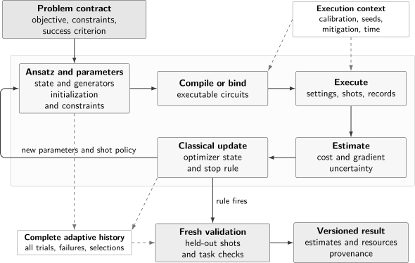

The hybrid loop is an adaptive experiment. Shot allocations, calibration context, seeds, mitigation, and stopping decisions affect the final estimator. Independent validation and a versioned result record are part of the algorithmic workflow, not optional presentation layers.

The distinction between symbolic parameters and executables matters. Changing $\boldsymbol{\theta}$ may only bind rotation angles in a fixed compiled template, or it may trigger new synthesis, routing, pulse generation, or calibration choices. The latter changes both cost and noise. A reproducible experiment records which operations were fixed across the loop and which were regenerated.

The optimizer is also part of the adaptive measurement policy. It determines which parameter points are queried and often how many shots are spent there. Consequently, one cannot generally treat all observations collected during training as independent, identically distributed samples from one fixed experiment.

Objective, Estimand, and Estimator

Three objects are easy to conflate:

1. the ideal objective defined by the mathematical problem;
2. the implemented estimand defined by the compiled circuit and physical experiment;
3. the finite-data estimator computed from observed records.

For an ideal pure-state objective,

$$C_{\mathrm{ideal}}(\boldsymbol{\theta}) = \operatorname{Tr} \left[ \rho_{\mathrm{ideal}}(\boldsymbol{\theta})O \right].$$

Compilation approximation and noise produce a physical state $\rho_{\mathrm{phys}}$, so the hardware estimand is

$$C_{\mathrm{phys}}(\boldsymbol{\theta},t) = \operatorname{Tr} \left[ \rho_{\mathrm{phys}}(\boldsymbol{\theta},t)O_{\mathrm{impl}} \right],$$

where $t$ denotes time-dependent context. A sample mean $\widehat C$ estimates $C_{\mathrm{phys}}$, not automatically $C_{\mathrm{ideal}}$. The useful decomposition is

$$\widehat C-C_{\mathrm{ideal}} = \bigl(\widehat C-C_{\mathrm{phys}}\bigr) + \bigl(C_{\mathrm{phys}}-C_{\mathrm{ideal}}\bigr).$$

The first term is statistical error. The second includes coherent miscalibration, decoherence, readout error, drift, compilation approximation, and any mismatch between the intended and realized observable. More shots reduce the first term but need not reduce the second.

Objectives built from many observables

Suppose

$$O = \sum_{a=1}^{M}w_a O_a, \qquad \mu_a(\boldsymbol{\theta}) = \langle O_a\rangle_{\boldsymbol{\theta}}.$$

With separately estimated terms,

$$\widehat C = \sum_{a=1}^{M}w_a\widehat\mu_a.$$

If term $a$ receives $N_a$ independent shots and its single-shot variance is $\sigma_a^2$, then, ignoring covariance between settings,

$$\operatorname{Var}(\widehat C) = \sum_{a=1}^{M} \frac{w_a^2\sigma_a^2}{N_a}.$$

For fixed total shots $N=\sum_a N_a$, the continuous optimum is

$$N_a \propto \lvert w_a\rvert\sigma_a.$$

Uniform allocation is therefore not generally optimal. In practice, $\sigma_a$ is unknown and can be learned from pilot data. Commuting terms can sometimes share measurement settings, but grouping introduces covariance and changes circuit count, basis-change depth, and statistical analysis. The measurement design must be optimized as a whole rather than term by term.

Nonlinear postprocessing

Ratios, logarithms, normalization by estimated quantities, postselected conditional means, and mitigation inverses can be biased at finite sample size. For a nonlinear map $g$,

$$\mathbb E[g(\widehat{\boldsymbol{\mu}})] \neq g(\mathbb E[\widehat{\boldsymbol{\mu}}])$$

in general. Bootstrap intervals can help with irregular estimators, but only if resampling respects the experimental hierarchy. Analytic propagation, likelihood methods, or simulation-based calibration may be preferable.

Parameterized Circuit Families

An ansatz is the map

$$\boldsymbol{\theta} \longmapsto \lvert\psi(\boldsymbol{\theta})\rangle.$$

Its reachable set is a manifold or stratified subset of state space, often of far lower dimension than the full Hilbert space. The key question is not whether the family can approximate arbitrary states, but whether it can reach useful states for the target instance at acceptable depth and can be searched with available precision.

Problem-inspired circuits

Problem-inspired ansatzes use generators, symmetries, conserved quantities, or known limiting states from the application. A layered form is

$$U(\boldsymbol{\theta}) = \prod_{\ell=1}^{L} \prod_{k=1}^{K} e^{-i\theta_{\ell k}G_k}.$$

If the generators commute with a symmetry $S$ and the initial state lies in one symmetry sector, then the circuit remains there:

$$[G_k,S]=0 \quad\Longrightarrow\quad [U(\boldsymbol{\theta}),S]=0.$$

This can exclude invalid states and reduce the search space. It can also exclude the solution if the sector, encoding, or assumed symmetry is wrong. Constraints should therefore be justified from the problem, not imposed only because they simplify optimization.

Hardware-efficient circuits

Hardware-efficient ansatzes alternate native single-qubit rotations and entangling layers chosen to match connectivity. They can minimize compiled depth for a given number of layers, but the phrase does not mean efficient optimization or favorable asymptotic scaling. Deep, highly random families can be expressive while producing concentrated costs and gradients. Native gates can also drift, crosstalk, and vary strongly across qubits.

Adaptive and growing circuits

An adaptive method adds generators or layers according to measured information. This can keep early circuits shallow and allocate parameters where they appear useful. It also creates a nested selection process: each proposed operator, gradient estimate, and stopping decision consumes measurements. Comparisons must count the rejected candidates and all intermediate circuits, not only the final compact ansatz.

Expressibility is not the objective

One expressibility diagnostic compares the distribution of state overlaps generated by the ansatz with the Haar distribution. Such metrics can rank circuit families, but closeness to Haar-random states is not synonymous with task performance. An ansatz may be:

• too restricted to represent the target;
• expressive enough for the target but easy to train;
• highly expressive yet redundant and statistically untrainable;
• expressive in ideal simulation but ineffective after noise.

The desired family is task sufficient, symmetry appropriate, compilable, and trainable under the actual estimator. Maximum generic expressibility is usually neither necessary nor desirable.

Exact Quantum Gradients

For

$$f(\theta) = \langle\psi_0\rvert U^\dagger(\theta)OU(\theta) \lvert\psi_0\rangle,$$

a derivative can often be written as a linear combination of expectation values evaluated by shifted circuits. This avoids differentiating sampled bit strings as though they were deterministic floating-point outputs.

Two-eigenvalue parameter-shift rule

Consider one gate

$$R_G(\theta) = e^{-i\theta G},$$

where the Hermitian generator $G$ has eigenvalues $\{-r,+r\}$. Holding all other gates fixed,

$$\frac{\partial f}{\partial\theta} = r \left[ f(\theta+s)-f(\theta-s) \right], \qquad s=\frac{\pi}{4r}.$$

For

$$R_P(\theta) = e^{-i\theta P/2}, \qquad P^2=I,$$

one has $r=1/2$ and therefore

$$\frac{\partial f}{\partial\theta} = \frac12 \left[ f\!\left(\theta+\frac{\pi}{2}\right) - f\!\left(\theta-\frac{\pi}{2}\right) \right].$$

This identity is exact for the ideal expectation function. Its finite-shot implementation remains a noisy gradient estimator. If one parameter controls several gates, the chain rule contributes once per occurrence unless a generalized rule exploits the full Fourier spectrum.

Generators with more than two distinct eigenvalues generally require more shifted evaluations or stochastic rules. Hardware noise can also make the implemented function differ from the ideal gate model. Parameter shift is not a universal two-circuit recipe independent of generator, compilation, and noise.

Gradient-estimator variance

If the two shifted costs are estimated independently with equal shot count and variance $v_\pm$, then the Pauli-rotation rule gives

$$\operatorname{Var}(\widehat{\partial_\theta f}) = \frac14 \left( v_++v_- \right).$$

Using common random numbers is not usually literal on hardware, because measurement outcomes from distinct quantum circuits are independent. Correlated calibration blocks or paired execution schedules can nevertheless reduce drift mismatch, and covariance must then be included explicitly.

For $p$ parameters, a naive full parameter-shift gradient can require order $2p$ objective evaluations per iteration, each of which may contain many measurement settings. This multiplicative cost is often more important than the nominal depth of one ansatz circuit.

Finite differences

The centered finite difference

$$\widehat g_j = \frac{ \widehat C(\boldsymbol{\theta}+h\mathbf e_j) - \widehat C(\boldsymbol{\theta}-h\mathbf e_j) }{2h}$$

has truncation bias of order $h^2$ for a smooth objective, while its sampling variance scales as order $1/(N h^2)$. Making $h$ smaller reduces truncation bias but amplifies shot noise, calibration quantization, and drift. A finite-difference step therefore requires an explicit bias-variance choice.

Simultaneous perturbation

Simultaneous perturbation stochastic approximation (SPSA) draws a random direction $\boldsymbol{\Delta}$, often with independent entries in $\{-1,+1\}$, and uses two cost evaluations:

$$\widehat g_j = \frac{ \widehat C(\boldsymbol{\theta}+c\boldsymbol{\Delta}) - \widehat C(\boldsymbol{\theta}-c\boldsymbol{\Delta}) }{2c\Delta_j}.$$

Its circuit-evaluation count does not grow linearly with $p$ per stochastic gradient estimate, but the estimate can have high variance and requires careful gain schedules. “Two evaluations” is not “two shots”: each cost may still require many circuits and measurements.

Classical Optimization

No optimizer is uniformly best for VQAs. The relevant regime combines noisy function evaluations, periodic parameters, constraints, heterogeneous curvature, device drift, expensive batches, and sometimes discrete ansatz choices.

First-order stochastic methods

An elementary update is

$$\boldsymbol{\theta}_{t+1} = \boldsymbol{\theta}_t - \eta_t\widehat{\boldsymbol g}_t.$$

Stochastic-gradient methods can converge with unbiased finite-variance estimators under regularity and step-size assumptions. VQA gradients may be estimated by sampling shots, observable terms, data records, or combinations of these. Such convergence statements do not guarantee reaching the global minimum of a nonconvex objective, and they do not rescue exponentially small signals.

Momentum and adaptive coordinate scaling can improve empirical behavior, but their hyperparameters and stopping rules are part of the algorithm. Tuning them on the reported instances without accounting for selection exaggerates performance.

Derivative-free methods

Nelder–Mead, Powell-type searches, coordinate methods, Bayesian optimization, and trust-region model building can be useful when gradients are unavailable or very noisy. Their decisions still depend on resolving cost differences. In a barren plateau those differences can be exponentially suppressed, so choosing a gradient-free optimizer does not by itself remove the information problem.

Curvature and trust regions

Quasi-Newton and trust-region methods use local models to adapt steps to curvature and uncertainty. They can reduce iteration count but may require additional evaluations, stable Hessian approximations, or bounds on model error. A noisy optimizer should reject or shrink a step when the predicted improvement is not statistically resolved, rather than treating every fluctuation as a descent direction.

Quantum Geometry and Natural Gradient

The same physical state can have many parameter descriptions, and equal Euclidean parameter steps need not represent equal changes in state. For a normalized pure-state family, the Fubini–Study metric is

$$g_{jk} = \operatorname{Re} \left[ \langle\partial_j\psi\vert\partial_k\psi\rangle - \langle\partial_j\psi\vert\psi\rangle \langle\psi\vert\partial_k\psi\rangle \right].$$

It defines the local line element

$$ds^2 = \sum_{j,k} g_{jk}\,d\theta_jd\theta_k.$$

For pure states, the quantum Fisher information matrix is $4g$ under a common convention. Because authors differ by this factor, an implementation should state which matrix it uses.

Quantum natural gradient chooses a step by solving

$$\left( g+\lambda I \right) \delta\boldsymbol{\theta} = - \eta\nabla C.$$

The regularizer $\lambda$ stabilizes directions in which $g$ is singular or poorly estimated. This update is invariant under smooth reparameterizations in the ideal geometric limit, unlike ordinary Euclidean gradient descent. Practical implementations often use diagonal or block-diagonal approximations.

Geometry is not free. Estimating $g$ can require additional circuits and shots, and inverting an ill-conditioned matrix amplifies estimator noise. The comparison that matters is total cost to a validated answer, not iterations to a low training objective.

Redundant parameters

If a nonzero vector $\boldsymbol v$ satisfies

$$g\boldsymbol v=0,$$

then the corresponding infinitesimal parameter displacement does not change the physical state to second order in the metric. Such null directions can come from repeated generators, circuit identities, symmetries, or state-dependent stabilizers. They create flat directions without necessarily creating a many-qubit barren plateau.

The effective local dimension is

$$d_{\mathrm{eff}} = \operatorname{rank}(g).$$

When $d_{\mathrm{eff}}<p$, reporting only the number of trainable parameters overstates the local capacity. Pruning redundant coordinates, tying parameters, or choosing a better chart can improve conditioning while leaving the reachable states unchanged locally.

Barren Plateaus

A barren plateau is a scaling phenomenon, not merely a plot that looks flat. For an ensemble of instances or random initializations, a common diagnostic is

$$\mathbb E_{\boldsymbol{\theta}} \left[ \partial_j C \right] = 0, \qquad \operatorname{Var}_{\boldsymbol{\theta}} \left[ \partial_j C \right] \in \mathcal O(b^{-n}),$$

for some $b>1$ as the number of qubits $n$ grows. Typical gradients then become exponentially small. Resolving their sign or relative size with incoherent sampling can require exponentially many measurements.

This definition is about a sequence of problem sizes and a specified sampling ensemble. A small gradient at one point may instead indicate a local optimum, a saddle, a symmetry, a redundant parameter, an insensitive observable, or a poor coordinate scale. Conversely, visibly nonzero gradients on eight qubits do not establish polynomial trainability.

Randomness and unitary designs

For sufficiently expressive randomly initialized circuits, parts of the circuit can approximate unitary 2-designs. Under the assumptions of the standard results, concentration of measure makes expectation gradients exponentially small. Depth, connectivity, gate ensemble, initial state, and observable all affect when that regime appears.

The lesson is not that every deep circuit has a barren plateau. It is that generic expressibility can erase the structured signal the optimizer needs. Random initialization should be treated as a substantive algorithmic choice.

Global and local costs

The support of the measured observable matters. Global costs can concentrate even for shallow circuits. In particular models, replacing a global fidelity- like objective with a sum of local costs changes exponential gradient scaling to polynomial scaling while preserving the same exact optimum.

That is not a universal license to localize every objective. A surrogate local cost must remain operational: low surrogate loss should imply success on the original task, with a quantitative bound if possible. Otherwise trainability is purchased by optimizing the wrong quantity.

Noise-induced plateaus

Noise contracts distinguishable states and can suppress both objective variation and gradients. For local unital Pauli noise, rigorous results show exponential gradient decay with circuit depth; when depth grows linearly with $n$, this becomes exponential in system size. Later analyses extend the picture to important nonunital channels and identify noise-induced limit sets as well as plateaus.

This mechanism differs from random-circuit concentration. A carefully initialized problem-inspired ansatz can still lose trainable signal as noisy depth grows. Error mitigation may reduce bias, but its sampling overhead and stability must be included before claiming that it restores trainability.

Gradient-free optimization does not evade concentration

Derivative-free methods compare nearby or modeled cost values. In a barren plateau, those differences are suppressed along with gradients. Resolving them still demands high precision. Changing optimizers can improve finite-size behavior, but it does not remove an information-theoretic signal-to-noise bottleneck.

Worst-case hardness

Training broad classes of variational algorithms is NP-hard in the worst case, even for some systems whose underlying quantum dynamics are classically tractable. This result rules out a universal efficient classical optimizer under standard complexity assumptions. It does not prove that every physical instance, ansatz, or initialization is hard. Complexity statements must retain their quantifiers.

Designing for Trainability

There is no single cure, but several design principles can improve the available signal.

Use structure before capacity

Choose initial states, generators, symmetries, and connectivity from the problem. Verify that the target is reachable in the chosen sector. Add depth only when a shallower family fails a prespecified approximation test.

Problem inspiration is not itself a proof against barren plateaus. The dynamical Lie algebra generated by the ansatz, the initial state, and the observable can still produce concentration. Numerical gradient scaling over a range of sizes is useful evidence, but a narrow range should not be fitted to an asymptotic law with false confidence.

Initialize near a meaningful map

Options include:

• parameters corresponding to a known limiting solution;
• identity-block initialization, where new gate blocks initially compose to the identity;
• parameter transfer from a nearby instance or smaller system;
• layerwise growth, with new layers initialized not to perturb the current state;
• restricted randomization around a structured point.

These methods can preserve initial gradients. They can also bias the search toward one basin, so multiple structured seeds and transparent failure reporting remain important.

Match the cost to the information scale

Prefer observables whose changes are resolvable at the available shot budget. Normalize weighted sums so that one large coefficient does not dominate optimizer scaling. If constraints are imposed through penalties,

$$C_\lambda = C_0 + \sum_r \lambda_r \langle A_r\rangle^2,$$

the penalties change curvature and measurement cost. A coefficient too small permits invalid states; one too large can make the landscape ill-conditioned. Report the chosen scale and a constraint-violation curve.

Grow precision with optimization

Early iterations may need only the direction of a large improvement. Late iterations may require enough shots to distinguish small changes. An adaptive policy can increase shots according to estimated variance, gradient norm, or trust-region acceptance.

For an estimated component $\widehat g_j$ with standard error $\operatorname{SE}(\widehat g_j)$, a simple signal diagnostic is

$$R_j = \frac{ \lvert\widehat g_j\rvert }{ \operatorname{SE}(\widehat g_j) }.$$

This ratio is not a universal stopping test, especially after selecting the largest component, but it exposes updates driven mainly by measurement noise. Prespecify how the shot budget changes when $R_j$ is small.

Noise, Drift, and Mitigation

On hardware, optimization targets the time-dependent implemented objective $C_{\mathrm{phys}}(\boldsymbol{\theta},t)$. If calibration changes during the loop, the optimizer sees a moving surface:

$$\frac{dC_{\mathrm{phys}}}{dt} = \nabla_{\boldsymbol{\theta}}C_{\mathrm{phys}} \cdot \dot{\boldsymbol{\theta}} + \left. \frac{\partial C_{\mathrm{phys}}}{\partial t} \right|_{\boldsymbol{\theta}}.$$

The first term on the right is intended optimization; the last term is drift. Interleaving reference circuits, randomizing execution order, and blocking paired parameter-shift circuits can help distinguish them. A single calibration snapshot before a long run is rarely enough to establish stationarity.

Noise can have several qualitatively different effects:

• bias: the minimum value and minimizer move;
• variance: shot-to-shot outcomes broaden;
• smoothing: high-frequency landscape features are attenuated;
• false structure: coherent errors introduce new parameter dependence;
• leakage or loss: the effective state space and retention probability change;
• nonstationarity: the objective changes during training.

Error mitigation changes the estimator. Readout correction, probabilistic error cancellation, zero-noise extrapolation, symmetry verification, and postselection have different assumptions and overheads. A mitigated objective can have lower bias and much larger variance. Optimization on mitigated values also creates adaptive selection effects. Report both raw and mitigated traces, the mitigation model, calibration data, effective sample overhead, and failure rules. The symmetry-verification specialist owns its projector, check, estimand, covariance, acceptance, and validation contract; this page retains hybrid-loop, gradient, trainability, optimizer, and algorithmic evidence ownership. See Noise in Quantum Information for the canonical noise taxonomy.

A One-Qubit Worked Example

Take

$$\lvert\psi(\theta)\rangle = R_y(\theta)\lvert0\rangle, \qquad C(\theta) = \langle Z\rangle_\theta.$$

The exact state is

$$\lvert\psi(\theta)\rangle = \cos\frac{\theta}{2}\lvert0\rangle + \sin\frac{\theta}{2}\lvert1\rangle,$$

so

$$C(\theta) = \cos\theta, \qquad \frac{dC}{d\theta} = -\sin\theta.$$

The parameter-shift rule returns

$$\begin{aligned} \frac12 \left[ C\!\left(\theta+\frac{\pi}{2}\right) - C\!\left(\theta-\frac{\pi}{2}\right) \right] &= \frac12 \left[ -\sin\theta-\sin\theta \right] \\ &= -\sin\theta. \end{aligned}$$

Each $Z$ measurement is a random variable $X\in\{-1,+1\}$ with

$$\operatorname{Var}(X) = 1-C(\theta)^2 = \sin^2\theta.$$

Near $\theta=0$, the gradient is small because this point is a maximum of the cost, not because of a barren plateau: there is no system-size scaling here. Near $\theta=\pi/2$, both shifted circuits have deterministic ideal outcomes, but hardware noise can reintroduce variance and bias. Even this trivial example separates exact calculus, shot statistics, and physical implementation.

Stopping and Validation

Common stopping rules include:

1. a fixed total resource budget;
2. a small estimated gradient with uncertainty accounted for;
3. no statistically resolved improvement over a window;
4. a trust-region radius below a threshold;
5. satisfaction of an independently meaningful target;
6. convergence of several seeds to compatible validated results.

Stopping when the observed cost first crosses a threshold is biased toward favorable noise fluctuations. Validate the selected point with fresh measurements and report the selection rule.

Minimum validation stack

A mature VQA study should include:

• exact or high-accuracy classical simulation at small sizes;
• analytically solvable limiting cases;
• comparison of ideal, sampled, noisy, and hardware objectives;
• fresh-shot re-evaluation of selected parameters;
• multiple seeds with all-run and failure statistics;
• at least one strong classical method under a comparable input-output contract;
• scaling in problem size, depth, parameter count, shots, and total time;
• raw and mitigated results when mitigation is used;
• checks of constraints, conserved quantities, and task-specific observables.

The Quantum Circuit Simulation page covers simulator roles, while Algorithmic Benchmarking owns broader benchmark design.

Do not validate only the training objective

A low objective can fail to imply useful output because the ansatz optimizes a surrogate, the estimator is biased, the selected point exploits noise, or the observable leaves important degrees of freedom unconstrained. Report task-level quantities that were not directly optimized. Examples include held-out observables, symmetry checks, approximation ratios, residual norms, or independent energy estimates.

Resource Accounting

Let iteration $t$ request circuit configurations $\mathcal C_t=\{c_{t1},\ldots,c_{tK_t}\}$ with shot counts $N_{tk}$. A basic quantum acquisition count is

$$N_{\mathrm{shots}} = \sum_t \sum_{k=1}^{K_t} N_{tk}.$$

This still omits rejected shots, resets, calibration, mitigation, queueing, and latency. An end-to-end decomposition is

$$\begin{aligned} T_{\mathrm{total}} &= T_{\mathrm{pre}} + T_{\mathrm{compile}} + T_{\mathrm{queue}} + T_{\mathrm{execute}} \\ &\quad + T_{\mathrm{classical}} + T_{\mathrm{validate}}. \end{aligned}$$

For a batch-access device, the number of quantum–classical round trips may dominate. Report:

• number of objective, gradient, metric, and validation evaluations;
• distinct executable circuits and total shots;
• circuit depth before and after routing;
• two-qubit gate count and measurement settings;
• optimizer iterations, seeds, restarts, and failed jobs;
• classical compute time and memory;
• QPU access time and end-to-end elapsed time;
• mitigation and calibration overhead;
• cost to the accepted result, not only cost of the winning run.

An empirical quantum advantage claim additionally requires a scaling study, a well-defined classical comparator, and uncertainty over representative instances. The Verification of Quantum Advantage page owns that stronger evidentiary standard.

The Quantum Algorithms and Complexity chapter guide places the complete hybrid ledger and evidence classification inside a matched algorithm claim before any speedup conclusion.

Classical Comparison

The appropriate comparator depends on the output contract. Possibilities include exact diagonalization, tensor networks, Monte Carlo, local search, convex relaxations, classical variational families, or domain-specific heuristics. “Classically hard in general” is not a benchmark.

Use the same:

• instance distribution and preprocessing;
• accuracy or task-quality target;
• success probability;
• inclusion or exclusion of warm starts;
• tuning budget and number of seeds;
• hardware and wall-clock boundary, or a clearly separated asymptotic model.

Small VQA instances are often deliberately classically simulable so that the experiment can be validated. That is scientifically useful, but it is not evidence of computational advantage. Conversely, failure to beat a classical method at small size does not prove asymptotic uselessness. State exactly which claim the evidence supports.

Common Mistakes

Calling every parameterized circuit a variational algorithm

A parameterized circuit becomes a VQA only when paired with a defined objective, estimation protocol, update rule, and output criterion. A circuit diagram alone is an ansatz.

Equating shallow depth with low total cost

Training may require thousands of circuit variants, measurement groups, and adaptive round trips. Depth is one resource coordinate.

Reporting the ideal objective as the hardware target

The device samples an implemented, noisy estimand. Separate statistical error from physical bias.

Treating parameter shift as noiseless differentiation

The identity is exact for the modeled expectation function; its experimental estimate has shot noise, drift, and model mismatch.

Maximizing expressibility

Approaching Haar-random behavior can worsen concentration and erase useful structure. Seek task-sufficient capacity.

Diagnosing a barren plateau from one flat trace

Barren plateaus are scaling statements over a specified ensemble. Check gradient distributions across sizes and rule out ordinary stationarity, symmetry, redundancy, and estimator resolution.

Hiding unsuccessful seeds

Best-of-many selection changes both expected performance and total cost. Report the full run distribution and selection rule.

Comparing optimizer iteration counts

One iteration may use two circuits, $2p$ shifted evaluations, a metric tensor, or a large Bayesian batch. Compare acquisition and end-to-end resources.

Validating on adaptively reused measurements

Fresh data are needed after choosing parameters, ansatz depth, mitigation settings, or the best checkpoint.

Inferring advantage from a decreasing cost

A descending training curve shows that one optimizer extracted some signal on one tested regime. Advantage requires a separate comparative scaling claim.

Where Variational Algorithms Are Used

VQAs appear in ground- and excited-state estimation, combinatorial optimization, dynamical simulation, linear-system objectives, state preparation, compilation, error correction, quantum machine learning, and metrology. These applications share hybrid optimization but differ in what their objectives certify.

The connection to Optimal Control is especially close: both optimize parameterized quantum evolution. Control usually treats physical pulse fields and dynamical constraints as primary, whereas circuit VQAs often treat a gate-level ansatz and an algorithmic objective as primary. The mathematical tools overlap, but their canonical engineering boundaries differ.

For reproducibility, archive the complete adaptive history, executable artifacts, environment, seeds, raw records, and analysis. The Reproducible Notebooks and Reporting Standards pages specify the broader artifact and provenance requirements.

Negative Results and Limitations places barren-plateau theorems, empirical trainability failures, classical reversals, and still-open utility claims in their proper logical categories.

Research Status

The hybrid variational architecture, parameter-shift calculus, and several barren-plateau mechanisms are established. Which structured ansatzes remain trainable and useful at scientifically relevant scale is not settled. Promising initialization, local-cost, adaptive-ansatz, geometry-aware, and shot-frugal methods have strong results in particular regimes, but no universal method removes representation error, nonconvex optimization, hardware noise, and measurement cost simultaneously.

Near-term demonstrations should therefore be described as empirical studies under explicit size, device, and budget conditions. Claims of scalability need measured or proved scaling; claims of utility need a task-level comparator; claims of advantage need end-to-end evidence. The absence of a known large-scale advantage is not a proof that all VQAs fail, and a successful small instance is not evidence that the obstacles disappear.

References

1. A. Peruzzo et al., “A variational eigenvalue solver on a photonic quantum processor,” Nature Communications 5, 4213 (2014), doi:10.1038/ncomms5213.
2. J. R. McClean, J. Romero, R. Babbush, and A. Aspuru-Guzik, “The theory of variational hybrid quantum-classical algorithms,” New Journal of Physics 18, 023023 (2016), doi:10.1088/1367-2630/18/2/023023.
3. J. Preskill, “Quantum computing in the NISQ era and beyond,” Quantum 2, 79 (2018), doi:10.22331/q-2018-08-06-79.
4. K. Mitarai, M. Negoro, M. Kitagawa, and K. Fujii, “Quantum circuit learning,” Physical Review A 98, 032309 (2018), doi:10.1103/PhysRevA.98.032309.
5. M. Schuld, V. Bergholm, C. Gogolin, J. Izaac, and N. Killoran, “Evaluating analytic gradients on quantum hardware,” Physical Review A 99, 032331 (2019), doi:10.1103/PhysRevA.99.032331.
6. M. Cerezo et al., “Variational quantum algorithms,” Nature Reviews Physics 3, 625–644 (2021), doi:10.1038/s42254-021-00348-9.
7. K. Bharti et al., “Noisy intermediate-scale quantum algorithms,” Reviews of Modern Physics 94, 015004 (2022), doi:10.1103/RevModPhys.94.015004.
8. D. Wierichs, J. Izaac, C. Wang, and C. Y.-Y. Lin, “General parameter-shift rules for quantum gradients,” Quantum 6, 677 (2022), doi:10.22331/q-2022-03-30-677.
9. L. Banchi and G. E. Crooks, “Measuring analytic gradients of general quantum evolution with the stochastic parameter shift rule,” Physical Review A 103, 052414 (2021), doi:10.1103/PhysRevA.103.052414.
10. R. Sweke et al., “Stochastic gradient descent for hybrid quantum-classical optimization,” Quantum 4, 314 (2020), doi:10.22331/q-2020-08-31-314.
11. J. M. Kübler, A. Arrasmith, L. Cincio, and P. J. Coles, “An adaptive optimizer for measurement-frugal variational algorithms,” Quantum 4, 263 (2020), doi:10.22331/q-2020-05-11-263.
12. J. Stokes, J. Izaac, N. Killoran, and G. Carleo, “Quantum natural gradient,” Quantum 4, 269 (2020), doi:10.22331/q-2020-05-25-269.
13. B. van Straaten and B. Koczor, “Measurement cost of metric-aware variational quantum algorithms,” PRX Quantum 2, 030324 (2021), doi:10.1103/PRXQuantum.2.030324.
14. S. Sim, P. D. Johnson, and A. Aspuru-Guzik, “Expressibility and entangling capability of parameterized quantum circuits for hybrid quantum-classical algorithms,” Advanced Quantum Technologies 2, 1900070 (2019), doi:10.1002/qute.201900070.
15. T. Haug, K. Bharti, and M. S. Kim, “Capacity and quantum geometry of parametrized quantum circuits,” PRX Quantum 2, 040309 (2021), doi:10.1103/PRXQuantum.2.040309.
16. Z. Holmes, K. Sharma, M. Cerezo, and P. J. Coles, “Connecting ansatz expressibility to gradient magnitudes and barren plateaus,” PRX Quantum 3, 010313 (2022), doi:10.1103/PRXQuantum.3.010313.
17. J. R. McClean, S. Boixo, V. N. Smelyanskiy, R. Babbush, and H. Neven, “Barren plateaus in quantum neural network training landscapes,” Nature Communications 9, 4812 (2018), doi:10.1038/s41467-018-07090-4.
18. M. Cerezo, A. Sone, T. Volkoff, L. Cincio, and P. J. Coles, “Cost function dependent barren plateaus in shallow parametrized quantum circuits,” Nature Communications 12, 1791 (2021), doi:10.1038/s41467-021-21728-w.
19. S. Wang et al., “Noise-induced barren plateaus in variational quantum algorithms,” Nature Communications 12, 6961 (2021), doi:10.1038/s41467-021-27045-6.
20. P. Singkanipa and D. A. Lidar, “Beyond unital noise in variational quantum algorithms: noise-induced barren plateaus and limit sets,” Quantum 9, 1617 (2025), doi:10.22331/q-2025-01-30-1617.
21. A. Arrasmith, M. Cerezo, P. Czarnik, L. Cincio, and P. J. Coles, “Effect of barren plateaus on gradient-free optimization,” Quantum 5, 558 (2021), doi:10.22331/q-2021-10-05-558.
22. M. Larocca et al., “Diagnosing barren plateaus with tools from quantum optimal control,” Quantum 6, 824 (2022), doi:10.22331/q-2022-09-29-824.
23. E. Grant, L. Wossnig, M. Ostaszewski, and M. Benedetti, “An initialization strategy for addressing barren plateaus in parametrized quantum circuits,” Quantum 3, 214 (2019), doi:10.22331/q-2019-12-09-214.
24. A. Skolik, J. R. McClean, M. Mohseni, P. van der Smagt, and M. Leib, “Layerwise learning for quantum neural networks,” Quantum Machine Intelligence 3, 5 (2021), doi:10.1007/s42484-020-00036-4.
25. L. Bittel and M. Kliesch, “Training variational quantum algorithms is NP-hard,” Physical Review Letters 127, 120502 (2021), doi:10.1103/PhysRevLett.127.120502.
26. J. C. Spall, “Multivariate stochastic approximation using a simultaneous perturbation gradient approximation,” IEEE Transactions on Automatic Control 37, 332–341 (1992), doi:10.1109/9.119632.
27. S. Endo, Z. Cai, S. C. Benjamin, and X. Yuan, “Hybrid quantum-classical algorithms and quantum error mitigation,” Journal of the Physical Society of Japan 90, 032001 (2021), doi:10.7566/JPSJ.90.032001.

Exercises

1. Derive the parameter-shift rule

Let

$$R_P(\theta) = e^{-i\theta P/2}, \qquad P^2=I.$$

Show directly that an expectation $f(\theta)$ is a trigonometric polynomial of the form $a+b\cos\theta+c\sin\theta$, and derive the two-point shift rule.

Solution

Because $P^2=I$,

$$R_P(\theta) = \cos\frac{\theta}{2}I - i\sin\frac{\theta}{2}P.$$

Substituting this expression and its adjoint around the observable produces terms proportional to $\cos^2(\theta/2)$, $\sin^2(\theta/2)$, and $\sin(\theta/2)\cos(\theta/2)$. Double-angle identities therefore give

$$f(\theta) = a+b\cos\theta+c\sin\theta.$$

Its derivative is

$$f'(\theta) = -b\sin\theta+c\cos\theta.$$

Meanwhile,

$$\frac12 \left[ f\!\left(\theta+\frac{\pi}{2}\right) - f\!\left(\theta-\frac{\pi}{2}\right) \right] = -b\sin\theta+c\cos\theta.$$

Thus the shifted expression equals $f'(\theta)$ exactly.

2. Allocate shots between observables

An objective is

$$C = 3\langle O_1\rangle - \langle O_2\rangle.$$

Pilot measurements estimate single-shot standard deviations $\sigma_1=0.4$ and $\sigma_2=0.9$. Allocate $10{,}000$ shots to minimize the variance when the terms are measured independently.

Solution

The continuous optimum obeys

$$N_a \propto \lvert w_a\rvert\sigma_a.$$

The weights are

$$3(0.4)=1.2, \qquad 1(0.9)=0.9.$$

Therefore

$$N_1 = 10000\frac{1.2}{2.1} \approx 5714,$$

and

$$N_2 \approx 4286.$$

Integer rounding can be adjusted to preserve the total. The derivation assumes independent settings and known stable variances; grouping or drift changes the allocation problem.

3. Separate bias from variance

A simulator predicts $C_{\mathrm{ideal}}=-1.20$. Hardware repetitions give $\widehat C=-1.05$ with standard error $0.01$. Explain what increasing the shot count by a factor of $100$ can and cannot establish.

Solution

Under independent stationary sampling, the standard error falls by a factor of $10$, to about $0.001$. This measures the hardware estimand more precisely. It does not force that estimand toward $-1.20$. The observed difference of $0.15$ may be physical bias from noise, compilation, readout, or drift. More shots distinguish a stable discrepancy more sharply but do not diagnose or remove it.

4. Identify a redundant parameter

Consider

$$U(\theta_1,\theta_2) = R_z(\theta_1)R_z(\theta_2)$$

acting on an arbitrary state. Find a null direction of the state-space metric.

Solution

Because rotations about the same axis compose,

$$U(\theta_1,\theta_2) = R_z(\theta_1+\theta_2).$$

Only the sum matters. The displacement

$$\delta\boldsymbol{\theta} = \epsilon(1,-1)$$

leaves the unitary exactly unchanged, so $(1,-1)$ is a null direction of the Fubini–Study metric for every input state. The two-coordinate model has at most one effective local dimension.

5. Diagnose a flat trace

A ten-qubit run shows nearly constant cost for 50 iterations. List four checks needed before calling this a barren plateau.

Solution

Check whether:

1. gradients and cost differences are below the estimator’s resolution;
2. the initialization is already near a stationary point;
3. symmetries or redundant parameters make the chosen directions inactive;
4. calibration drift or optimizer step sizes obscure genuine changes.

Then study gradient distributions over initializations and a sequence of problem sizes. A barren-plateau claim requires exponential scaling under a specified ensemble, not one flat optimization history.

6. Count a naive gradient batch

An objective has 40 independently measured groups. A circuit has 120 parameters, each appearing in one Pauli rotation. A full parameter-shift gradient uses 2,000 shots per group and shifted point. How many shots does one gradient batch use?

Solution

There are two shifted points per parameter, so the number of group evaluations is

$$2(120)(40) = 9600.$$

At 2,000 shots each,

$$N_{\mathrm{shots}} = 9600(2000) = 19{,}200{,}000.$$

This excludes the unshifted objective, metric estimation, calibration, validation, rejected trials, and repeated seeds. The example shows why circuit depth alone is a poor proxy for VQA cost.

7. Audit best-of-seed reporting

A study runs 30 seeds, validates only the seed with the lowest noisy training cost, and reports that validation score as typical performance. What is wrong, and what should be reported?

Solution

The chosen seed is an order statistic selected after noisy evaluation. Validating that seed with fresh data removes reuse bias for its score, but it does not make the seed typical. Report all seeds, convergence and failure rates, the distribution of fresh validation scores, the prespecified selection rule, and the total cost of 30 runs. If the operational workflow intentionally uses best-of-30, report its performance as such and include all 30-run cost.

8. Design a stopping rule under shot noise

Propose a stopping rule for a noisy VQA that is more defensible than “stop after three iterations without a lower observed cost.”

Solution

One option is to maintain a trust region and estimate the improvement of the candidate over the incumbent using paired execution blocks. Stop when, for a prespecified number of accepted or attempted steps, the upper confidence bound on improvement is below a practical threshold and the remaining shot budget cannot resolve a smaller target improvement. Also stop at a fixed global budget. Re-evaluate the selected incumbent with fresh shots afterward.

The exact interval method and threshold must be declared in advance, and the analysis must account for repeated adaptive comparisons. The rule distinguishes “no detectable useful improvement” from “three noisy values happened not to decrease.”