Hybrid Quantum Simulation

Hybrid quantum simulation deliberately composes quantum and classical representations, or distinct modes of quantum control, so that each component handles a part of a specified simulation task. The word hybrid describes the architecture of the workflow. It does not imply low depth, near-term utility, variational optimization, or freedom from error.

Three families account for most uses of the term:

1. Digital–analog simulation interleaves continuously parameterized native many-body evolution with discrete gates or pulses.
2. Variational quantum–classical simulation estimates a projected equation of motion or objective on a quantum device and updates a compact state representation classically.
3. Quantum embedding assigns a correlated fragment or impurity to a quantum solver while a classical environment supplies boundary data and enforces a closure or self-consistency condition.

These families can overlap. A variational impurity solver may itself use digital–analog control. A digital–analog state-preparation block may sit inside a larger classical feedback loop. Classification is useful only when it makes the interfaces, resources, and failure modes more explicit.

This page is the canonical home for those hybrid interfaces: what crosses each boundary, how approximation and estimator errors feed back, when a loop has converged, and what must be validated end to end. What Is Quantum Simulation? owns the general simulation contract. Digital Quantum Simulation and Analog Quantum Simulation own the two execution paradigms separately. Variational Quantum Algorithms owns generic objectives, gradients, optimizer geometry, and barren plateaus; VQE owns the Rayleigh–Ritz ground-energy problem.

The Interface Contract

A hybrid workflow should be specified as a composition of maps rather than by a list of hardware components. One useful abstract contract is

$$\mathfrak H = \left( \mathcal M_Q, \mathcal M_C, I_{C\to Q}, I_{Q\to C}, \mathcal S, \mathcal V, \epsilon, \delta \right).$$

Here:

• $\mathcal M_Q$ is the family of quantum states, channels, or native evolutions used by the quantum component;
• $\mathcal M_C$ is the classical model, parameterization, or environment;
• $I_{C\to Q}$ translates classical parameters into circuits, pulse schedules, Hamiltonians, or boundary conditions;
• $I_{Q\to C}$ turns measurement records into classical estimators;
• $\mathcal S$ is the scheduler or update rule, including stopping criteria;
• $\mathcal V$ is the validation procedure;
• $\epsilon$ and $\delta$ are the requested accuracy and failure probability for a declared output.

The contract is incomplete unless it identifies the target model, initial state, observable family, parameter regime, and resource boundary inherited from the general simulation task. In particular, a hybrid method does not automatically return a wavefunction. Its output may be an observable estimate, a parameter trajectory, a self-consistent Green’s function, a fragment density matrix, or a prepared state.

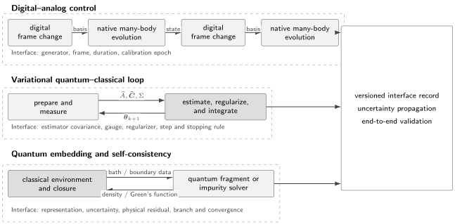
The three principal hybrid architectures place their boundaries in different locations. A trustworthy implementation records the maps, conventions, uncertainties, calibration context, and stopping rule at every boundary; the label hybrid alone supplies none of these guarantees.

What must cross a boundary

Every interface should have a machine-checkable data contract. Depending on the architecture, a record may include:

Field	Examples	Why it matters
quantity	pulse duration, angle, expectation value, Green’s function, density matrix	identifies the mathematical object being exchanged
basis and ordering	qubit map, orbital order, Pauli convention, frequency grid	prevents silent representation mismatches
units and scale	radians, angular frequency, energy, target-to-lab time factor	distinguishes a correct number from a correctly interpreted number
uncertainty	standard error, covariance, confidence region, systematic bound	allows downstream propagation rather than point-estimate reuse
provenance	circuit hash, pulse version, calibration epoch, seed, mitigation rule	makes adaptive runs reproducible and drift auditable
validity domain	parameter range, symmetry sector, subspace, bath discretization	prevents extrapolation beyond the calibrated map
acceptance rule	residual threshold, budget, held-out check, maximum iterations	separates stopping from retrospective judgment

Covariance is especially easy to lose. If several observables are estimated from the same shots, calibration fit, or randomized measurement ensemble, they are generally correlated. A classical update that treats them as independent can report a misleading parameter uncertainty even when every marginal error bar is correct.

Hybrid is a topology, not a quality label

The following statements do not follow from the architecture:

• a digital–analog sequence has less error than a gate-only circuit;
• a short variational circuit is trainable or classically intractable;
• a converged embedding loop represents the full material accurately;
• moving work to a classical computer lowers end-to-end cost;
• a quantum subroutine is responsible for the scientific performance.

Each is an empirical or mathematical claim requiring its own assumptions. A hybrid workflow can be an excellent engineering choice because it exploits a native interaction, reduces coherent depth, or isolates a strongly correlated subproblem. It can also exchange one bottleneck for many adaptive measurements, unstable feedback, or a hard-to-validate model boundary.

Digital–Analog Quantum Simulation

A digital–analog simulator composes native many-body evolutions with discrete control operations. Let $H_j(\boldsymbol\lambda_j)$ be a calibrated native Hamiltonian available for duration $\tau_j$, and let $D_j$ denote a discrete gate layer or fast control pulse. A general sequence has the form

$$U_{\mathrm{DA}} = D_m e^{-iH_m\tau_m/\hbar} \cdots D_2 e^{-iH_2\tau_2/\hbar} D_1 e^{-iH_1\tau_1/\hbar}.$$

The continuously tunable entangling evolutions are the analog blocks; the discrete operations select frames, refocus terms, alter signs, permute degrees of freedom, or compose blocks into a broader model family. The sequence may be open loop. No classical optimizer is required for this use of hybrid.

Toggling frames

Conjugating an available block by a digital operation changes its generator:

$$D e^{-iH\tau/\hbar}D^\dagger = e^{-i(DHD^\dagger)\tau/\hbar}.$$

This identity is the basic mechanism behind sign reversal, basis changes, and Hamiltonian refocusing. If a hardware interaction supplies $ZZ$ couplings, single-qubit rotations can turn them into $XX$ or $YY$ couplings. Local $X$ pulses can reverse selected $Z$ fields or selected Ising bonds. The useful question is not whether the native block is universal by itself, but which target generators lie in the control algebra generated by the available blocks and discrete operations at acceptable cost.

Product composition and noncommutativity

For two bounded generators $A$ and $B$, a short block pair obeys the Baker–Campbell–Hausdorff expansion

$$\begin{aligned} e^{-iA\Delta t/\hbar} e^{-iB\Delta t/\hbar} &= \exp\!\left[ -\frac{i\Delta t}{\hbar}(A+B) -\frac{\Delta t^2}{2\hbar^2}[A,B] +O(\Delta t^3) \right]. \end{aligned}$$

Thus the effective generator is

$$H_{\mathrm{eff}} = A+B -\frac{i\Delta t}{2\hbar}[A,B] +O(\Delta t^2).$$

Noncommuting blocks therefore introduce a controllable composition error much like a product formula. That algorithmic error is distinct from mismatch in the physical generators $A$ and $B$. Increasing the number of blocks can reduce the former while increasing exposure to pulse error, drift, leakage, and decoherence.

The abstract order conditions belong on Trotter Product Formula, while Trotter–Suzuki Methods develops simulation-level commutator bounds, ordering, cost, and refinement tests. Here the important point is architectural: a nominally exact analog block does not make the composed sequence exact.

Worked example: an exact refocusing block

Suppose the native two-qubit Hamiltonian is

$$H = J Z_1Z_2 +h_1Z_1 +h_2Z_2.$$

Let $P=X_1X_2$. Because $XZX=-Z$,

$$PHP = JZ_1Z_2 -h_1Z_1 -h_2Z_2.$$

All terms are diagonal in the computational basis, so $H$ and $PHP$ commute. The echo sequence

$$U_{\mathrm{echo}}(\tau) = P e^{-iH\tau/(2\hbar)} P e^{-iH\tau/(2\hbar)}$$

is therefore exactly

$$\begin{aligned} U_{\mathrm{echo}}(\tau) &= e^{-i(PHP)\tau/(2\hbar)} e^{-iH\tau/(2\hbar)} \\ &= e^{-iJZ_1Z_2\tau/\hbar}. \end{aligned}$$

Under the ideal model, the local fields cancel with no product-formula error while the interaction survives. In a laboratory, finite pulse duration can allow $H$ to act during $P$; pulse-axis error can leave residual fields; extra $XX$, $ZX$, or spectator couplings may not commute; and the two half-intervals may see different drift. The exact algebra establishes the intended block, not its physical fidelity.

Stepwise and always-on control

In a stepwise protocol, analog interactions are nominally switched on and off between digital layers. In an always-on or banged protocol, fast digital pulses are applied while a background interaction continues to act. The latter can avoid switching transients, but the digital and analog controls then overlap. An instantaneous-pulse model must be replaced by a time-ordered Hamiltonian,

$$U(T) = \mathcal T \exp\!\left[ -\frac{i}{\hbar} \int_0^T \bigl(H_{\mathrm{native}}+H_{\mathrm{ctrl}}(t)\bigr) \,dt \right].$$

Whether one version is better is hardware- and task-dependent. Switching errors, bandwidth, pulse distortions, crosstalk, and analog-block calibration must enter the comparison alongside circuit depth.

A digital–analog error ledger

For a target unitary $U_\star$, a useful decomposition is

$$\epsilon_{\mathrm{DA}} \lesssim \epsilon_{\mathrm{synth}} +\epsilon_{\mathrm{model}} +\epsilon_{\mathrm{pulse}} +\epsilon_{\mathrm{noise}} +\epsilon_{\mathrm{SPAM}},$$

where the symbol $\lesssim$ signals that the terms need not be independent or strictly additive for the chosen metric. The entries mean:

• synthesis error: the ideal sequence differs from the target operation;
• model error: the inferred native generator differs from the physical one;
• pulse error: finite-bandwidth digital controls fail to implement their assumed frame transformations;
• noise error: decoherence, stochastic control variation, loss, and leakage;
• SPAM error: state-preparation and measurement bias in the final estimate.

For ideal unitary blocks with operator-norm errors $\epsilon_j$, a telescoping argument gives the conservative bound

$$\left\| \widetilde U_m\cdots\widetilde U_1 -U_m\cdots U_1 \right\| \le \sum_{j=1}^{m}\epsilon_j.$$

This is not a prediction that every error adds linearly. Coherent errors can cancel or align, stochastic errors can accumulate differently, and observable- specific error can be much smaller. The bound does show why counting native blocks without characterizing them is not a resource or accuracy estimate.

Variational Quantum Simulation

Variational quantum simulation compresses a state or process into a parameterized manifold and uses measured quantities to choose its motion. It is different from merely optimizing a final energy: the classical update is intended to approximate a differential equation for real time, imaginary time, or an open-system process.

Let

$$\lvert\psi(\boldsymbol\theta)\rangle \in \mathcal M$$

be a normalized ansatz with real parameters $\theta_i$. Exact Schrödinger evolution generally points outside the tangent space of $\mathcal M$. A variational principle projects the exact velocity onto the accessible tangent directions, after removing the physically irrelevant global phase.

Phase-invariant tangent projection

Define the projective tangent vectors

$$\lvert D_i\psi\rangle = \left( I-lvert\psi\rangle\langle\psi\rvert \right) \lvert\partial_i\psi\rangle,$$

and the instantaneous energy

$$E = \langle\psi\rvert H\lvert\psi\rangle.$$

McLachlan projection minimizes the norm of the projective residual

$$\lvert R\rangle = \sum_j \dot\theta_j \lvert D_j\psi\rangle +\frac{i}{\hbar} (H-E) \lvert\psi\rangle.$$

Stationarity with respect to each real velocity $\dot\theta_i$ gives

$$\sum_j A_{ij}\dot\theta_j = C_i,$$

with

$$\begin{aligned} A_{ij} &= \operatorname{Re} \langle D_i\psi\vert D_j\psi\rangle, \\ C_i &= \frac{1}{\hbar} \operatorname{Im} \langle D_i\psi\rvert H\lvert\psi\rangle. \end{aligned}$$

$A$ is the real part of the quantum geometric tensor on the ansatz manifold. It is positive semidefinite and can be singular when parameters are redundant or locally inactive. Some presentations fix a phase convention instead of using $\lvert D_i\psi\rangle$ explicitly; sign and gauge conventions must be kept consistent when formulas are combined.

At one time step, the hybrid loop is:

1. prepare $\lvert\psi(\boldsymbol\theta_k)\rangle$;
2. estimate the required entries of $A$ and $\boldsymbol C$;
3. solve a regularized linear system for $\dot{\boldsymbol\theta}_k$;
4. integrate to $\boldsymbol\theta_{k+1}$;
5. repeat, while evaluating validation observables and stopping conditions.

The general design of ansatzes, gradients, shot allocation, and optimizers is covered by Variational Quantum Algorithms. The distinctive issue here is whether a measured tangent projection tracks the target dynamics over time.

Projection error is a physical diagnostic

The minimum local residual

$$\epsilon_{\mathrm{proj}}(t) = \min_{\boldsymbol v} \left\| \sum_j v_j\lvert D_j\psi\rangle +\frac{i}{\hbar}(H-E)\lvert\psi\rangle \right\|$$

measures how much of the exact projective velocity lies outside the ansatz tangent space. A small optimization residual for the linear solve is not the same quantity. One can solve $A\dot{\boldsymbol\theta}=\boldsymbol C$ perfectly even when the ansatz manifold misses most of the target velocity.

The local projection residual is also not the entire trajectory error. Time integration, finite sampling, regularization, hardware bias, and repeated feedback can accumulate. Observable-specific checks along the path remain necessary.

Worked example: exact one-qubit motion

Take

$$H = \frac{\hbar\Omega}{2}Z, \qquad \lvert\psi(\theta)\rangle = e^{-i\theta Z/2} \lvert +x\rangle.$$

Because $\langle Z\rangle=0$ on this orbit,

$$\lvert D_\theta\psi\rangle = -\frac{i}{2}Z\lvert\psi\rangle.$$

The scalar metric and force are

$$A = \frac14, \qquad C = \frac{1}{\hbar} \operatorname{Im} \langle D_\theta\psi\rvert H\lvert\psi\rangle = \frac{\Omega}{4}.$$

Therefore $\dot\theta=\Omega$, exactly matching Schrödinger evolution. The ansatz is invariant under the target Hamiltonian, so $\epsilon_{\mathrm{proj}}=0$. A finite-step Euler update still introduces integration error for general observables or nonlinear parameterizations, and measured estimates of $A$ and $C$ still carry uncertainty. Exact representability does not make an implementation exact.

Ill-conditioning amplifies estimator error

Suppose measurements return

$$\widehat A=A+\delta A, \qquad \widehat{\boldsymbol C} = \boldsymbol C+\delta\boldsymbol C.$$

To first order, the velocity perturbation obeys

$$\delta\dot{\boldsymbol\theta} \approx A^+ \left( \delta\boldsymbol C -\delta A\,\dot{\boldsymbol\theta} \right),$$

where $A^+$ is the Moore–Penrose pseudoinverse on retained tangent directions. Consequently,

$$\left\| \delta\dot{\boldsymbol\theta} \right\| \lesssim \left\|A^+\right\| \left( \left\|\delta\boldsymbol C\right\| + \left\|\delta A\right\| \left\|\dot{\boldsymbol\theta}\right\| \right).$$

Near-null tangent directions make $\lVert A^+\rVert$ large. Truncating small eigenvalues, adding Tikhonov regularization, or constraining the step can reduce variance, but each changes the projected dynamics and introduces bias. The threshold is therefore part of the algorithm, not a numerical footnote.

Real time, imaginary time, and general processes

For normalized imaginary-time evolution with inverse-energy coordinate $\tau$,

$$\frac{d}{d\tau} \lvert\psi\rangle = -(H-E)\lvert\psi\rangle,$$

the same tangent projection yields

$$\sum_j A_{ij}\dot\theta_j = -\operatorname{Re} \langle D_i\psi\rvert H\lvert\psi\rangle.$$

Imaginary-time projection can prepare low-energy states, but finite ansatz capacity, normalization, conditioning, and measurement cost still control its quality. VQE is the canonical home for static variational energy guarantees.

Variational principles can also be formulated for density operators, purifications, stochastic trajectories, and general linear processes. In those settings, preserving trace, Hermiticity, positivity, and complete positivity may require more than minimizing a Hilbert-space residual. A low-residual parameter trajectory is not by itself a certificate that every intermediate object is a physical state or channel.

The variational dynamics error budget

A useful trajectory-level ledger separates

$$\epsilon_{\mathrm{traj}} \lesssim \epsilon_{\mathrm{ansatz}} +\epsilon_{\mathrm{projection}} +\epsilon_{\mathrm{estimation}} +\epsilon_{\mathrm{solve}} +\epsilon_{\mathrm{integration}} +\epsilon_{\mathrm{hardware}}.$$

These labels distinguish:

• inability of the ansatz family to represent relevant states;
• local tangent-space mismatch;
• finite-shot and readout uncertainty in $A$ and $\boldsymbol C$;
• regularization and numerical linear-solve error;
• finite-step propagation error;
• preparation, gate, drift, leakage, and mitigation bias.

The terms interact. Hardware bias changes the estimated vector field; the classical integrator then repeatedly follows that biased field. Reducing circuit depth can therefore be offset by the number and adaptivity of measurements needed to reconstruct it.

Quantum Embedding and Self-Consistency

Quantum embedding assigns a selected correlated region to a quantum solver and represents the rest of the system through a classical environment. The full Hamiltonian may be partitioned schematically as

$$H = H_F +H_E +H_{FE},$$

where $F$ denotes a fragment or impurity and $E$ its environment. The method does not usually discard $E$. It compresses the environment into boundary data such as a bath hybridization, self-energy, correlation potential, mean field, or reduced density matrix.

An abstract embedding loop is

$$\begin{aligned} H_{\mathrm{imp}}^{(k)} &= \mathcal B\!\left[x_k\right], \\ \widehat y_k &= \mathcal Q\!\left[H_{\mathrm{imp}}^{(k)}\right], \\ x_{k+1} &= \mathcal F\!\left(x_k,\widehat y_k\right). \end{aligned}$$

$\mathcal B$ constructs the finite quantum problem from classical environment data $x_k$. The quantum solver $\mathcal Q$ returns observables $\widehat y_k$. The classical closure $\mathcal F$ updates the environment. At convergence, the selected fragment and environment quantities satisfy a prescribed matching condition.

DMFT and DMET illustrate different interfaces

In dynamical mean-field theory (DMFT), a lattice problem is mapped to an interacting impurity coupled to a self-consistent bath. The exchanged objects are frequency- or time-dependent Green’s functions, hybridization functions, and self-energies. The mapping is exact in the infinite-coordination limit for the class of models covered by the theory, but practical calculations still have impurity-solver, bath-discretization, statistical, and continuation errors.

Density matrix embedding theory (DMET) instead uses a frequency-independent one-particle density matrix and a finite bath derived from an auxiliary state. The closure and observables differ from DMFT. Calling both methods “an impurity loop” is not enough to make their guarantees interchangeable.

A proposed quantum-accelerated embedding workflow can use a quantum processor as the impurity solver while retaining classical density-functional, mean-field, DMFT, or DMET machinery around it. The quantum processor then addresses a selected correlated subproblem. It does not directly simulate all electrons in the bulk material, and the embedding approximation remains part of the scientific error budget.

Fixed-point stability

Write the ideal deterministic update as

$$x_{k+1}=G(x_k),$$

with fixed point $x_\star=G(x_\star)$. Suppose $G$ is a contraction in a declared norm over the relevant region,

$$\left\| G(x)-G(z) \right\| \le L\lVert x-z\rVert, \qquad 0\le L<1,$$

and each implemented update has bounded perturbation $\lVert\xi_k\rVert\le\eta$:

$$\widehat x_{k+1} = G(\widehat x_k)+\xi_k.$$

Then

$$\begin{aligned} \left\| \widehat x_k-x_\star \right\| &\le L^k \left\| \widehat x_0-x_\star \right\| \\ &\quad+ \eta \frac{1-L^k}{1-L}. \end{aligned}$$

The asymptotic error floor is at most $\eta/(1-L)$. Near a weakly stable fixed point with $L\approx1$, small quantum-estimator or fitting errors can be strongly amplified. This bound is illustrative rather than universal: many embedding maps are not globally contractive, may have multiple solutions, and can be non-normal in their linearized dynamics.

Mixing changes stability, not the fixed point

A common damped update is

$$x_{k+1} = (1-\lambda)x_k +\lambda G(x_k), \qquad 0<\lambda\le1.$$

For a scalar map, local stability at $x_\star$ requires

$$\left| 1-\lambda +\lambda G'(x_\star) \right|<1.$$

Smaller $\lambda$ can stabilize an oscillatory update, but it also makes the raw iterate difference

$$\left|x_{k+1}-x_k\right| = \lambda \left|G(x_k)-x_k\right|$$

artificially small. A stopping test should inspect the unmixed physical residual $\lVert G(x_k)-x_k\rVert$, not only successive iterate changes.

In several dimensions, the Jacobian spectrum controls local asymptotic stability, while non-normality can produce large transient amplification even when every eigenvalue lies inside the unit disk. Monitoring only a final fixed-point residual can miss that sensitivity.

Worked example: bias amplification in a scalar closure

Consider

$$G(x)=ax+c, \qquad |a|<1.$$

The ideal fixed point is

$$x_\star = \frac{c}{1-a}.$$

If the quantum solver contributes a persistent additive bias $b$, the implemented map is $\widetilde G(x)=ax+c+b$, and its apparently well-converged fixed point is

$$\widetilde x_\star = x_\star +\frac{b}{1-a}.$$

For $a=0.9$ and $b=10^{-3}$, the final bias is $10^{-2}$. The iteration can converge smoothly to many decimal places while being ten times more biased than the quantum subroutine’s local offset. Convergence certifies consistency with the implemented map, not correctness of that map.

Embedding-specific approximation layers

An embedding result may depend on all of the following:

• choice and size of the correlated fragment or active space;
• bath construction and discretization;
• environment approximation and exchange-correlation functional;
• interaction parameters and double-counting correction;
• impurity state preparation and solver error;
• real- or imaginary-frequency grid and Fourier transforms;
• analytic continuation when real-frequency spectra are inferred;
• statistical error, covariance, and nonlinear fitting;
• branch selection, initialization, mixing, and stopping rule.

Increasing the accuracy of the quantum impurity solver cannot remove errors from the surrounding model. Conversely, a useful embedding approximation may not require a uniformly precise impurity state if the requested fragment observable is robust. Accuracy should be allocated to the final scientific quantity.

Unified Feedback Error Propagation

Variational and embedding workflows can both be written locally as

$$\begin{aligned} \widehat y_k &= Q(x_k)+b_k+\eta_k, \\ x_{k+1} &= F(x_k,\widehat y_k), \end{aligned}$$

where $b_k$ is systematic bias and $\eta_k$ is a random estimator error. Near a reference trajectory, first-order perturbation gives

$$\delta x_{k+1} = J_k\delta x_k +B_k b_k +B_k\eta_k,$$

with

$$J_k = \frac{\partial F}{\partial x} +\frac{\partial F}{\partial y} \frac{\partial Q}{\partial x}, \qquad B_k = \frac{\partial F}{\partial y}.$$

This equation exposes three separate questions:

1. Stability: do perturbations in the current classical state decay or grow under $J_k$?
2. Interface sensitivity: how strongly does the update react to measured quantities through $B_k$?
3. Estimator quality: what are the bias and covariance of the actual quantum output?

For a stationary linearized map $J$ with spectral radius below one, a persistent bias produces the steady displacement

$$\delta x_{\mathrm{bias}} = (I-J)^{-1}B b.$$

If independent zero-mean noise has covariance $\Sigma_\eta$, the stationary state covariance, when it exists, satisfies the discrete Lyapunov equation

$$\Sigma_x = J\Sigma_xJ^{\mathsf T} +B\Sigma_\eta B^{\mathsf T}.$$

The mean and covariance answer different questions. More shots can reduce the random term but not a fixed readout, model, or mitigation bias. Correlated drift violates the independent-noise assumption and can masquerade as physical movement of the classical state.

Digital–analog open-loop sequences do not have the same classical feedback, but coherent block errors propagate through conjugation by subsequent unitaries. In every family, the order and sensitivity of composition matter; subroutine error bars cannot simply be pasted onto the final answer.

Resource Accounting

Hybrid methods often shorten one coherent quantum execution by repeating it many times. A transparent resource statement reports both axes.

For adaptive iteration $k$, let $m_k$ be the number of measurement settings and $n_{ka}$ the shots assigned to setting $a$. The total shots are

$$N_{\mathrm{shots}} = \sum_{k=1}^{K} \sum_{a=1}^{m_k} n_{ka}.$$

This number should be accompanied by:

• quantum systems or logical qubits and any ancillas;
• native analog evolution time and control bandwidth;
• digital gate counts, depth, and two-qubit or multiqubit blocks;
• reset, preparation, readout, and calibration executions;
• number of adaptive round trips and optimizer or embedding restarts;
• classical memory, linear algebra, tensor contractions, fitting, and preprocessing;
• compilation, queue, communication, and data-analysis latency;
• failed, discarded, and postselected executions.

A schematic wall-clock model is

$$\begin{aligned} T_{\mathrm{wall}} \approx \sum_{k=1}^{K} \Bigg[ &T_{\mathrm{compile}}^{(k)} +T_{\mathrm{queue}}^{(k)} +T_{\mathrm{classical}}^{(k)} \\ &+ \sum_{a=1}^{m_k} n_{ka} T_{\mathrm{cycle}}^{(k,a)} \Bigg]. \end{aligned}$$

Measurement settings within one iteration may be parallelized, but adaptive iterations generally lie on a critical path. A method with shallow circuits can be slow when it requires thousands of sequential quantum–classical round trips. Conversely, a native analog block may reduce gate count while requiring expensive Hamiltonian characterization over a large control region.

Compare against the right classical boundary

A claim of quantum benefit should include all classical work that is necessary to construct and interpret the quantum subproblem. For embedding, that may include electronic-structure preprocessing and self-consistency. For variational dynamics, it includes metric estimation, regularization, integration, and repeated compilation. For digital–analog simulation, it includes pulse optimization and generator identification.

The comparison should use the best applicable classical method for the same target observable, accuracy, and input access. A quantum fragment solver must be compared with modern classical impurity solvers, not with brute-force simulation of the entire material. A short trajectory must be compared with tensor-network, Monte Carlo, semiclassical, or problem-specific methods in the regime where they apply.

Validation and Stopping

A hybrid workflow needs tests at three scales:

1. Component tests validate native blocks, circuits, estimators, classical solvers, and update rules independently.
2. Interface tests check basis conventions, units, covariance propagation, serialization, and sensitivity to exchanged quantities.
3. End-to-end tests compare final observables with exact limits, independent methods, held-out data, or experimentally known constraints.

Validation interventions

Useful interventions include:

• solve small instances exactly and compare the entire trajectory, not only its endpoint;
• halve a time step, tighten a regularizer, enlarge an ansatz, or increase a fragment and look for controlled convergence;
• replace measured quantum data with exact simulated interface data to isolate the classical loop;
• replay recorded quantum data through alternative classical updates;
• test symmetries, conservation laws, positivity, causality, and sum rules;
• reserve observables that are not used for fitting or stopping;
• interleave reference circuits or calibration blocks to expose drift;
• compare branches from multiple initializations and report the selection rule;
• perturb interface data within its covariance and propagate the full result.

For digital–analog protocols, turning off selected refocusing pulses can test the inferred Hamiltonian terms. For variational dynamics, compare the measured projection residual with held-out observables and step-size convergence. For embedding, vary fragment size, bath representation, mixing, and initial branch while monitoring physical residuals.

A stopping rule is not a certificate

A robust stopping rule combines several conditions, for example:

$$\begin{aligned} \lVert r_k\rVert &\le \tau_r, \\ \left| \widehat O_k-\widehat O_{k-1} \right| &\le \tau_O, \\ \operatorname{SE}(\widehat O_k) &\le \tau_{\mathrm{stat}}, \end{aligned}$$

for a required number of consecutive iterations, together with a maximum budget. The residual $r_k$ must be defined in physical, unmixed variables. Repeated estimates used in an adaptive run are correlated, so the standard error of a difference should include covariance.

Meeting these conditions establishes that the implemented loop has stopped according to its declared rule. It does not establish low model error, uniqueness of the solution, or agreement with the target system. Those require validation evidence beyond the stopping data.

Evidence ladder

From weakest to strongest, a hybrid simulation claim may be supported by:

1. an internally consistent output trace;
2. convergence under shots, step size, regularization, or iteration count;
3. agreement with exact small instances and solvable limits;
4. agreement of held-out observables or conservation laws;
5. cross-method or cross-platform agreement in overlapping regimes;
6. calibrated error propagation to the target observable;
7. useful predictions outside the fitted regime that survive independent tests;
8. an end-to-end resource advantage at matched accuracy.

These are different achievements. A converged variational trace is not a certified trajectory, and a verified trajectory is not yet a practical advantage demonstration.

Choosing a Hybrid Architecture

Scientific or engineering constraint	Architecture that may help	Main price paid
a calibrated many-body interaction is much cheaper than decomposing it	digital–analog blocks	hardware-specific synthesis and generator uncertainty
target dynamics remain near a compact parameterized manifold	variational projection	repeated metric and force estimation, projection bias, conditioning
strong correlations are localized to a fragment or active space	quantum embedding	environment approximation, boundary matching, self-consistency
coherence time is scarce but repeated preparation is available	variational or embedding loop	shot count, latency, and feedback bias
model parameters must change widely	digital gates or variational controls	compilation or retraining cost
direct access to large analog systems is available	analog or digital–analog protocol	restricted model family and validation burden

The architecture should follow the target bottleneck. Hybridization for its own sake adds interfaces, and every interface is another place where conventions, uncertainty, or causality can be lost.

Common Mistakes

Calling every pulse-level circuit digital–analog

All physical gates arise from continuous control. The term is informative when the algorithm deliberately exposes a continuously parameterized multiqubit evolution as a native block, rather than treating it only as a compiled fixed gate.

Counting blocks but not their calibration

A many-body block may replace many two-qubit gates while requiring extensive Hamiltonian learning, crosstalk correction, or restricted operating points. Report characterization cost and validity range.

Equating a solved linear system with accurate dynamics

A tiny residual in $A\dot{\boldsymbol\theta}=\boldsymbol C$ says the measured projected equation was solved. It does not bound tangent-space mismatch, trajectory accumulation, or hardware bias.

Regularizing silently

Eigenvalue truncation and damping stabilize an ill-conditioned update by changing it. Report the threshold, retained rank, sensitivity, and resulting bias checks.

Declaring convergence from successive mixed iterates

Heavy mixing makes $x_{k+1}-x_k$ small by construction. Evaluate the unmixed closure residual and physical observables.

Treating finite-shot error as the only uncertainty

More shots do not remove calibration bias, model inadequacy, ansatz error, branch ambiguity, bath discretization, or faulty interface conventions.

Comparing with an irrelevant classical baseline

The correct baseline solves the same task at matched accuracy using all applicable structure. Exponential Hilbert-space dimension is not by itself an end-to-end advantage argument.

Reusing adaptive data as independent validation

Measurements that selected parameters, mixing, ansatz growth, or stopping are training data. Reserve held-out observables, instances, or execution blocks for validation.

Research Status

Digital–analog control, variational principles, DMFT, and DMET are established frameworks. Their mathematical foundations and many small- and intermediate- scale demonstrations are well developed. The architecture-dependent limits are equally important.

As of 2026, digital–analog simulation remains strongly hardware-specific: native multiqubit interactions can reduce compiled depth, but complete comparisons must include control overlap, calibration, and model error. Variational real- and imaginary-time simulation remains active research in ansatz design, metric estimation, regularization, long-time stability, and certifiable error bounds. Quantum-accelerated embedding remains a promising route to correlated materials, but projected resource estimates and proof-of- principle calculations do not yet establish broad practical advantage over the best classical impurity and embedding methods.

There is no general theorem that hybridizing a simulation improves accuracy or complexity. The durable result is more modest and more useful: exposing a problem’s natural interfaces can reduce the quantum task, provided that the interfaces themselves are stable, measured, and validated.

Key Results

• Hybrid simulation is an interface architecture, not an error or performance guarantee.
• Digital–analog control composes native many-body evolution with discrete frame changes; noncommuting blocks carry synthesis error in addition to physical generator error.
• Variational dynamics projects the exact vector field onto an ansatz tangent space. The projection residual and the conditioning of the quantum metric are independent diagnostics.
• Embedding replaces a large environment with boundary data and a closure condition. Convergence of that condition does not remove fragment, bath, or environment-model error.
• Feedback can amplify both bias and variance. Near a linear fixed point, the factors $(I-J)^{-1}$ and the Lyapunov equation quantify that sensitivity.
• Resource accounting must include native evolution, gates, shots, adaptive round trips, calibration, and classical computation.
• Component validation, interface validation, and end-to-end validation answer different questions and are all required for strong claims.

References

1. I. M. Georgescu, S. Ashhab, and F. Nori, “Quantum simulation,” Reviews of Modern Physics 86, 153–185 (2014), doi:10.1103/RevModPhys.86.153.
2. A. Parra-Rodriguez, P. Lougovski, L. Lamata, E. Solano, and M. Sanz, “Digital-analog quantum computation,” Physical Review A 101, 022305 (2020), doi:10.1103/PhysRevA.101.022305.
3. T. Gonzalez-Raya et al., “Digital-analog quantum simulations using the cross-resonance effect,” PRX Quantum 2, 020328 (2021), doi:10.1103/PRXQuantum.2.020328.
4. I. Arrazola, J. S. Pedernales, L. Lamata, and E. Solano, “Digital-analog quantum simulation of spin models in trapped ions,” Scientific Reports 6, 30534 (2016), doi:10.1038/srep30534.
5. Y. Li and S. C. Benjamin, “Efficient variational quantum simulator incorporating active error minimization,” Physical Review X 7, 021050 (2017), doi:10.1103/PhysRevX.7.021050.
6. X. Yuan, S. Endo, Q. Zhao, Y. Li, and S. C. Benjamin, “Theory of variational quantum simulation,” Quantum 3, 191 (2019), doi:10.22331/q-2019-10-07-191.
7. S. McArdle, T. Jones, S. Endo, Y. Li, S. C. Benjamin, and X. Yuan, “Variational ansatz-based quantum simulation of imaginary time evolution,” npj Quantum Information 5, 75 (2019), doi:10.1038/s41534-019-0187-2.
8. S. Endo, J. Sun, Y. Li, S. C. Benjamin, and X. Yuan, “Variational quantum simulation of general processes,” Physical Review Letters 125, 010501 (2020), doi:10.1103/PhysRevLett.125.010501.
9. A. D. McLachlan, “A variational solution of the time-dependent Schrödinger equation,” Molecular Physics 8, 39–44 (1964), doi:10.1080/00268976400100041.
10. C. Kokail et al., “Self-verifying variational quantum simulation of lattice models,” Nature 569, 355–360 (2019), doi:10.1038/s41586-019-1177-4.
11. M. Cerezo et al., “Variational quantum algorithms,” Nature Reviews Physics 3, 625–644 (2021), doi:10.1038/s42254-021-00348-9.
12. A. B. Magann et al., “From pulses to circuits and back again: a quantum optimal control perspective on variational quantum algorithms,” PRX Quantum 2, 010101 (2021), doi:10.1103/PRXQuantum.2.010101.
13. A. Georges, G. Kotliar, W. Krauth, and M. J. Rozenberg, “Dynamical mean-field theory of strongly correlated fermion systems and the limit of infinite dimensions,” Reviews of Modern Physics 68, 13–125 (1996), doi:10.1103/RevModPhys.68.13.
14. G. Kotliar et al., “Electronic structure calculations with dynamical mean-field theory,” Reviews of Modern Physics 78, 865–951 (2006), doi:10.1103/RevModPhys.78.865.
15. G. Knizia and G. K.-L. Chan, “Density matrix embedding: a simple alternative to dynamical mean-field theory,” Physical Review Letters 109, 186404 (2012), doi:10.1103/PhysRevLett.109.186404.
16. B. Bauer, D. Wecker, A. J. Millis, M. B. Hastings, and M. Troyer, “Hybrid quantum-classical approach to correlated materials,” Physical Review X 6, 031045 (2016), doi:10.1103/PhysRevX.6.031045.
17. J. M. Kreula, S. R. Clark, and D. Jaksch, “Non-linear quantum-classical scheme to simulate non-equilibrium strongly correlated fermionic many-body dynamics,” Scientific Reports 6, 32940 (2016), doi:10.1038/srep32940.
18. A. J. Daley et al., “Practical quantum advantage in quantum simulation,” Nature 607, 667–676 (2022), doi:10.1038/s41586-022-04940-6.
19. J. R. McClean, J. Romero, R. Babbush, and A. Aspuru-Guzik, “The theory of variational hybrid quantum-classical algorithms,” New Journal of Physics 18, 023023 (2016), doi:10.1088/1367-2630/18/2/023023.
20. S. Endo, Z. Cai, S. C. Benjamin, and X. Yuan, “Hybrid quantum-classical algorithms and quantum error mitigation,” Journal of the Physical Society of Japan 90, 032001 (2021), doi:10.7566/JPSJ.90.032001.

Further Connections

• What Is Quantum Simulation? defines the common target-model correspondence, output contract, error budget, and evidence ladder.
• Digital Quantum Simulation develops the gate-based representation, algorithm, compilation, execution, and readout stack.
• Analog Quantum Simulation develops effective-Hamiltonian reduction, parameter maps, leakage, readout, and analog validation.
• Simulation of Quantum Materials applies variational, digital–analog, and embedding interfaces to periodic and effective materials models with workflow-wide resource and validation requirements.
• Variational Quantum Algorithms owns generic hybrid objectives, finite-shot estimation, gradients, trainability, and optimizer validation.
• VQE owns variational ground-energy estimation and the Rayleigh–Ritz guarantee.
• Optimal Control connects pulse-level control, differentiable evolution, robust objectives, and closed-loop calibration.
• Materials Simulation Case Studies compares model, material, observable, validation, and resource claims for concrete applications.
• Reporting Standards specifies the provenance and uncertainty records needed to audit adaptive experiments.

Exercises

1. Classify interfaces, not labels

Classify each workflow and identify the quantity crossing its principal interface:

1. fixed single-qubit rotations alternate with tunable all-to-all Ising evolution;
2. a circuit estimates a tangent-space metric and a classical integrator updates circuit angles;
3. a quantum processor returns an impurity Green’s function used to update a classical bath;
4. a classically optimized pulse implements a fixed gate and is then used without feedback in an otherwise digital circuit.

Solution

1. This is digital–analog simulation. The interface inside the quantum control sequence exchanges frame choices, pulse labels, and native-block durations.
2. This is variational quantum–classical simulation. Estimated entries of $A$ and $\boldsymbol C$, with covariance, cross from quantum execution to the classical integrator; updated angles return.
3. This is quantum embedding. A Green’s function crosses to the classical bath update, and new bath or hybridization parameters return.
4. The offline use of classical pulse optimization does not by itself make the simulation hybrid in the architectural sense used here. Every implemented gate has classical control. The executed simulation is digital unless the optimized pulse is exposed as a continuously parameterized analog block or enters an adaptive quantum–classical loop.

2. Verify the two-qubit echo

For

$$H=JZ_1Z_2+h_1Z_1+h_2Z_2,$$

show explicitly that the echo sequence in the text cancels both local fields. Would $P=X_1$ cancel the same terms?

Solution

Conjugation by $P=X_1X_2$ gives

$$PZ_1P=-Z_1, \qquad PZ_2P=-Z_2, \qquad PZ_1Z_2P=Z_1Z_2.$$

Because all three Pauli strings commute,

$$U_{\mathrm{echo}} = \exp\!\left[ -\frac{i\tau}{2\hbar}(PHP+H) \right] = e^{-iJZ_1Z_2\tau/\hbar}.$$

For $P=X_1$, both $Z_1$ and $Z_1Z_2$ change sign while $Z_2$ does not. That echo would cancel the interaction and the $h_1Z_1$ term but retain $h_2Z_2$.

3. Derive the leading composition term

Use the Baker–Campbell–Hausdorff formula to find the leading correction to the effective Hamiltonian of $e^{-iA\Delta t/\hbar}e^{-iB\Delta t/\hbar}$. Explain why the correction is Hermitian when $A$ and $B$ are Hermitian.

Solution

Set $X=-iA\Delta t/\hbar$ and $Y=-iB\Delta t/\hbar$. Then

$$\log(e^Xe^Y) = X+Y+\frac12[X,Y]+O(\Delta t^3).$$

Since

$$[X,Y] = -\frac{\Delta t^2}{\hbar^2}[A,B],$$

comparison with $-iH_{\mathrm{eff}}\Delta t/\hbar$ gives

$$H_{\mathrm{eff}} = A+B -\frac{i\Delta t}{2\hbar}[A,B] +O(\Delta t^2).$$

For Hermitian $A$ and $B$, the commutator is anti-Hermitian, so $-i[A,B]$ is Hermitian.

4. Derive the projected real-time equation

Starting from

$$\lvert R\rangle = \sum_j\dot\theta_j\lvert D_j\psi\rangle +\frac{i}{\hbar}(H-E)\lvert\psi\rangle,$$

minimize $\langle R\vert R\rangle$ with respect to real $\dot\theta_i$. Recover $A\dot{\boldsymbol\theta}=\boldsymbol C$.

Solution

For real velocities,

$$\frac12 \frac{\partial}{\partial\dot\theta_i} \langle R\vert R\rangle = \operatorname{Re} \langle D_i\psi\vert R\rangle.$$

Stationarity gives

$$\sum_j \operatorname{Re} \langle D_i\psi\vert D_j\psi\rangle \dot\theta_j +\operatorname{Re} \left[ \frac{i}{\hbar} \langle D_i\psi\rvert H\lvert\psi\rangle \right] =0.$$

The energy term vanishes because $\langle D_i\psi\vert\psi\rangle=0$. Using $\operatorname{Re}(iz)=-\operatorname{Im}(z)$ gives

$$\sum_j A_{ij}\dot\theta_j = \frac{1}{\hbar} \operatorname{Im} \langle D_i\psi\rvert H\lvert\psi\rangle =C_i.$$

5. Diagnose a singular variational metric

Let

$$A= \begin{pmatrix} 1&0\\ 0&10^{-6} \end{pmatrix}, \qquad \boldsymbol C= \begin{pmatrix} 1\\ 10^{-3} \end{pmatrix}.$$

Find the unregularized velocity. If the uncertainty in $C_2$ is $2\times10^{-4}$, find its contribution to the uncertainty in $\dot\theta_2$. What changes if eigenvalues below $10^{-5}$ are truncated?

Solution

Direct inversion gives

$$\dot{\boldsymbol\theta} = \begin{pmatrix} 1\\ 10^3 \end{pmatrix}.$$

The standard uncertainty propagated from $C_2$ alone is

$$\sigma_{\dot\theta_2} = \frac{2\times10^{-4}}{10^{-6}} =200.$$

The small metric eigenvalue amplifies both the force and its noise. Truncating eigenvalues below $10^{-5}$ sets the second pseudoinverse component to zero, so the retained solution is $(1,0)^{\mathsf T}$. Its variance is lower, but it has deliberately removed motion along the second direction. Whether that bias is acceptable must be tested against trajectory observables.

6. Prove the contraction error floor

Assume $G$ has contraction factor $L<1$ and

$$\widehat x_{k+1}=G(\widehat x_k)+\xi_k, \qquad \lVert\xi_k\rVert\le\eta.$$

Derive the finite-$k$ error bound relative to the ideal fixed point.

Solution

Let $e_k=\lVert\widehat x_k-x_\star\rVert$. Since $x_\star=G(x_\star)$,

$$e_{k+1} \le L e_k+\eta.$$

Iterating the recursion gives

$$e_k \le L^k e_0 +\eta\sum_{j=0}^{k-1}L^j = L^k e_0 +\eta\frac{1-L^k}{1-L}.$$

Thus $\limsup_{k\to\infty}e_k\le\eta/(1-L)$. The result requires a uniform deterministic perturbation bound and contraction in the chosen norm; it should not be applied unchanged to unstable or multibranch maps.

7. Analyze damping and a deceptive residual

For $G(x)=-2x+c$, determine the range of $\lambda$ for which

$$x_{k+1}=(1-\lambda)x_k+\lambda G(x_k)$$

is locally stable. Explain why $|x_{k+1}-x_k|$ alone becomes a poor stopping diagnostic as $\lambda\to0$.

Solution

The derivative of the mixed map is

$$1-\lambda+\lambda(-2) = 1-3\lambda.$$

Stability requires

$$|1-3\lambda|<1,$$

so $0<\lambda<2/3$. Meanwhile,

$$x_{k+1}-x_k = \lambda\bigl(G(x_k)-x_k\bigr).$$

For very small $\lambda$, successive iterates can be nearly equal even when the unmixed fixed-point residual $G(x_k)-x_k$ is large. The stopping rule should examine the latter or divide out the known mixing factor.

8. Design an end-to-end validation study

A variational quantum impurity solver is inserted into a classical embedding loop. List a minimal set of experiments that separately test the quantum solver, the classical closure, the interface, and the final material observable.

Solution

A defensible study would include at least:

1. exact or high-accuracy classical comparisons for small impurity instances, including held-out observables and covariance calibration;
2. a run of the classical closure with exact synthetic impurity data, testing branch dependence, mixing, and the unmixed residual;
3. round-trip interface tests for orbital ordering, units, symmetries, frequency grids, and uncertainty propagation;
4. shot, mitigation, regularization, bath, and fragment-size convergence;
5. multiple initializations with a prespecified branch-selection rule;
6. comparison of final held-out material observables with an independent method or controlled limit;
7. an end-to-end resource record including failed and calibration executions.

No single test substitutes for the others. A precise impurity solver cannot validate the embedding approximation, and a converged embedding loop cannot validate a biased quantum estimator.