Digital Quantum Simulation

Digital quantum simulation uses a programmable sequence of discrete quantum operations to approximate the states, dynamics, spectra, or observables of a specified quantum model. The target degrees of freedom are encoded into qubits or qudits; the target generator is represented through implementable operators or access oracles; a simulation algorithm produces a logical circuit; that circuit is compiled to a device; and repeated measurements produce a classical estimate of the requested quantity.

The word digital describes the control interface, not the scientific output. A digital simulator does not print an exponentially long wavefunction. It returns samples, expectation values, correlation functions, eigenvalue estimates, or a prepared quantum state whose useful properties must still be measured. Nor does universality make every simulation efficient. State preparation, long-time evolution, controlled access, native compilation, fault tolerance, and output extraction can each dominate the cost.

This page is the canonical home for the gate-based simulation workflow: representation, state preparation, evolution-algorithm choice, Pauli-string compilation, observable extraction, physical execution, error allocation, and validation. What Is Quantum Simulation? owns the broader digital–analog–hybrid taxonomy and scientific simulation contract. Hybrid Quantum Simulation owns the composition of native many-body blocks with digital frame changes, as well as variational and embedding interfaces. Trotter Product Formula owns the operator identity and derivation. Algorithmic Primitives owns the abstract Hamiltonian-access, block-encoding, and signal-processing interfaces. Those results are used here to explain an executable workflow, not rederived in full.

The End-to-End Task

A closed-system dynamical task can be specified by

$$\mathfrak T = \left( H, \rho_0, \mathcal O, \mathcal T, \epsilon, \delta \right),$$

where $H$ is the target Hamiltonian, $\rho_0$ the initial state, $\mathcal O$ a declared observable set, $mathcal T$ a set or interval of times, $epsilon$ an accuracy target, and $delta$ an allowed failure probability. For $O\in\mathcal O$, the ideal quantity may be

$$\mu_O(t) = \operatorname{Tr} \left[ Oe^{-iHt}\rho_0e^{iHt} \right],$$

using units with $\hbar=1$ unless restored explicitly.

A complete digital simulation must specify procedures for:

1. mapping the target Hilbert space into finite registers;
2. constructing or accessing the encoded Hamiltonian;
3. preparing an encoded approximation to $\rho_0$;
4. approximating $e^{-iHt}$, or another target channel, to a stated error;
5. compiling the logical operations into an allowed gate set and topology;
6. measuring enough records to estimate the requested outputs;
7. quantifying algorithmic, physical, statistical, and model errors;
8. validating the result where an independent check is possible.

Leaving any one of these as “given” changes the claim from an end-to-end simulation algorithm to a conditional subroutine result.

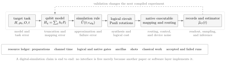
A digital simulation crosses several non-equivalent interfaces. Query complexity constrains the simulation-rule box; logical gate counts constrain the circuit box; native depth and noise constrain execution; and measurement cost constrains the estimator. A defensible result carries errors, resources, and validation evidence across the entire stack.

What Universality Establishes

For a broad class of local Hamiltonians

$$H = \sum_{\ell=1}^{L}H_\ell,$$

where each $H_\ell$ acts on only a bounded number of subsystems and has an efficient description, a universal gate-based quantum computer can approximate the corresponding finite-time evolution with resources polynomial in system size, time, and inverse accuracy under the assumptions of the chosen algorithm. This is the central content of universal digital simulation.

It does not establish that:

• an arbitrary dense matrix supplied as a classical table can be loaded efficiently;
• an unknown ground state can be prepared efficiently;
• evolution for exponentially long physical time can generically be compressed into polynomial cost;
• every target observable can be estimated with polynomially many shots;
• physical gate errors remain bounded without mitigation or fault tolerance;
• the best classical method for the requested output is exponentially slow.

For generic black-box Hamiltonians, no-fast-forwarding results show that cost must grow at least linearly with simulated time in the worst case. Structured exceptions exist: commuting models, known spectra, free systems, fast-forwardable families, and tasks involving restricted observables can be easier. The correct statement is model- and access-dependent, not “quantum evolution is always exponentially faster.”

From a Target Model to Qubits

The first computational decision is a representation. An isometry

$$V: \mathcal H_{\rm tar}^{(\rm trunc)} \longrightarrow (\mathbb C^2)^{\otimes n}$$

embeds a finite target subspace into $n$ qubits. The encoded Hamiltonian and observables are

$$H_q = V H_{\rm trunc}V^\dagger, \qquad O_q = V O_{\rm trunc}V^\dagger,$$

on the code subspace. Choosing $V$ determines qubit count, operator locality, symmetry visibility, circuit depth, and readout complexity.

Distinguishable local systems

A spin-$1/2$ degree of freedom maps directly to one qubit. A local system of dimension $d$ can use $\lceil\log_2 d\rceil$ qubits in a compact binary encoding, or more qubits in a unary or one-hot encoding. Compact encodings save qubits but may turn local operators into longer Pauli strings. Redundant encodings can make constraints and transitions simpler to implement.

Bosonic modes require a cutoff, basis, and encoding. A number cutoff $n_{\max}$ replaces an infinite-dimensional Fock space by dimension $n_{\max}+1$. The resulting truncation error is physical and state-dependent; it is not a gate error. Convergence must be demonstrated by increasing the cutoff or bounding the omitted population.

Fermions and constraints

Fermionic creation and annihilation operators cannot be replaced naively by local qubit raising and lowering operators because anticommutation signs must be preserved. Jordan–Wigner, parity, and Bravyi–Kitaev-style maps trade Pauli weight, parity bookkeeping, and circuit structure differently. Jordan–Wigner Transformation owns the canonical one-dimensional mapping and its strings.

Gauge constraints, fixed particle number, parity, and point-group sectors can be handled by an encoding that satisfies them identically, by penalty terms, or by detection and postprocessing. These choices are not equivalent. A penalty Hamiltonian changes the spectrum and introduces another energy scale; postselection changes sampling cost; symmetry-preserving encodings can reduce the accessible Hilbert space but complicate gates.

Pauli representation

Every $n$-qubit Hermitian operator has a Pauli expansion

$$H_q = \sum_{\ell=1}^{L}h_\ell P_\ell, \qquad P_\ell \in \{I,X,Y,Z\}^{\otimes n},$$

with real coefficients

$$h_\ell = \frac{1}{2^n} \operatorname{Tr}(P_\ell H_q).$$

The formal upper bound is $L\leq4^n$, so a Pauli expansion is useful only when the target structure makes it sparse, compressible, or efficiently queryable. A polynomial number of local terms is very different from an arbitrary list of exponentially many Pauli strings.

State Preparation Is Part of the Algorithm

Digital evolution begins from a state, not from a Hamiltonian alone. Easy inputs include computational-basis product states, simple stabilizer states, and shallow states created by known local rotations. Harder tasks include interacting ground states, thermal states, scattering wave packets, and states with topological or gauge constraints.

Common preparation routes include:

• direct basis-state or low-depth circuit preparation;
• adiabatic interpolation from an easy Hamiltonian;
• variational preparation with a classical optimization loop;
• dissipative or measurement-based preparation;
• spectral filtering or phase estimation from a trial state;
• postselection into a symmetry or energy sector.

If the desired eigenstate is $|E_0\rangle$ and the prepared trial state is

$$|\psi_{\rm trial}\rangle = \sqrt p,|E_0\rangle + \sqrt{1-p}\,|E_\perp\rangle,$$

then an ideal projective energy measurement produces the desired energy only with probability $p$. Repetition costs order $1/p$ preparations unless an additional coherent amplification or filtering method is available. Quantum Phase Estimation owns this spectral-overlap and controlled-evolution analysis.

Preparation quality should be tied to the final task. If the actual and ideal initial states have trace distance

$$D(\rho_0,\widetilde\rho_0) = \frac12 \lVert\rho_0-\widetilde\rho_0\rVert_1,$$

then ideal unitary evolution preserves that distance, and every bounded observable satisfies

$$\left| \operatorname{Tr} \left[ O(\rho_t-\widetilde\rho_t) \right] \right| \leq 2\lVert O\rVert_\infty D(\rho_0,\widetilde\rho_0).$$

This gives a rigorous task-independent conversion from state-preparation error to observable error. A much smaller observable-specific error may be possible, but it must be demonstrated rather than assumed.

Choosing a Digital Evolution Method

The Hamiltonian representation determines which simulation methods are available. There is no universally best algorithm after logical gates, ancillas, constants, connectivity, and output cost are included.

Method family	Input or access model	Main strength	Main cost or caveat
product formulas	exponentials of terms $H_\ell$	direct circuits, few ancillas, exploits commutation and locality	step error and term ordering; depth grows with step count
randomized formulas	sampled implementable terms	can reduce dependence on term count and coherent ordering bias	produces a randomized channel and requires seed/variance accounting
LCU and truncated Taylor methods	efficient linear combination of unitaries	strong precision dependence and coherent error control	state preparation, select operations, ancillas, and amplification
qubitization and QSP	block encoding with normalization $\alpha$	near-optimal dependence on $\alpha t$ and precision	constructing controlled block-encoding oracles may dominate
variational compilation	trainable circuit and objective	shallow task-specific approximation on available hardware	optimization, generalization, certification, and training cost
fault-tolerant synthesis	logical access to the chosen method	controllably small logical error	code cycles, magic states, routing, and physical-qubit overhead

Product formulas

For a time-independent sum $H=\sum_{\ell=1}^{L}H_\ell$, a first-order step is

$$S_1(\Delta t) = \prod_{\ell=1}^{L} e^{-iH_\ell\Delta t},$$

and $r$ steps approximate the target evolution:

$$e^{-iHt} \approx S_1(t/r)^r.$$

The error vanishes when the relevant terms commute. For bounded operators, a coarse first-order bound has the structure

$$\left\| e^{-iHt} - S_1(t/r)^r \right\| \lesssim \frac{t^2}{2r} \sum_{j<k} \lVert[H_j,H_k]\rVert,$$

up to higher-order contributions and convention-dependent refinements. Modern bounds exploit nested commutators, locality, ordering, and the target observable; simply replacing every term by its norm can be extremely loose.

The symmetric second-order step

$$S_2(\Delta t) = \left( \prod_{\ell=1}^{L} e^{-iH_\ell\Delta t/2} \right) \left( \prod_{\ell=L}^{1} e^{-iH_\ell\Delta t/2} \right)$$

has global error of order $t^3/r^2$ under standard boundedness assumptions, with constants governed by nested commutators. Higher-order formulas trade more exponentials per step for a higher power of $1/r$. The exact derivation, domain qualifications, and Suzuki recursion belong to Trotter Product Formula.

Randomized compilation

Randomization can turn coherent, ordering-dependent approximation error into a controlled average channel. For a Pauli sum, define

$$\lambda = \sum_{\ell=1}^{L}|h_\ell|, \qquad p_\ell = \frac{|h_\ell|}{\lambda}.$$

The qDRIFT protocol independently samples index $\ell$ with probability $p_\ell$ and applies

$$U_\ell = \exp \left[ -i\,operatorname{sgn}(h_\ell) \frac{\lambda t}{N_s}P_\ell \right]$$

for each of $N_s$ random steps. Its average-channel error can be bounded with $N_s$ scaling as order $\lambda^2t^2/\epsilon$ in the basic analysis, independent of the explicit term count $L$. This can help when $L$ is large but $\lambda$ is moderate. It is not free: circuit-to-circuit randomness, hardware error, statistical variance, and the distinction between an average channel and each sampled realization must be included.

Linear-combination and qubitization methods

Suppose the encoded Hamiltonian is available through an $(\alpha,a,\epsilon_{\rm BE})$ block encoding $U_H$ satisfying

$$\left\| H - \alpha \left( \langle0^a|\otimes I \right) U_H \left( |0^a\rangle\otimes I \right) \right\| \leq \epsilon_{\rm BE}.$$

Qubitization converts this access into invariant two-dimensional signal subspaces, and quantum signal processing applies a polynomial approximation to the desired exponential. The resulting query complexity can be nearly linear in $\alpha t$ and near-logarithmic in $1/\epsilon$ in appropriate regimes.

That statement is conditional on the block-encoding interface. The costs of preparing coefficient states, implementing the select oracle, uncomputing ancillas, controlling the operation, and synthesizing QSP phases must be expanded into gates before comparing with a product formula. A worse normalization $\alpha$ directly worsens the query count. Hamiltonian Simulation owns access models, normalized-time complexity, method selection, generic no-fast-forwarding limits, and output-specific guarantees. Qubitization and Quantum Signal Processing owns the signal-subspace construction, admissible evolution polynomials, QSP phase conventions, approximation ledger, and oracle-to-gate expansion.

Time-dependent generators

For $H(t)$, the target is a time-ordered exponential

$$U(t,0) = \mathcal T \exp \left[ -i\int_0^t ds\,H(s) \right].$$

Freezing $H$ on time slices introduces discretization error even before terms within a slice are split. Dyson-series, Magnus, interaction-picture, and time-dependent product-formula methods use different smoothness and access assumptions. A method proven for a static Hamiltonian cannot simply be applied to a fast drive without adding the time-discretization error and oracle cost.

Compiling Pauli Evolution

Fix the convention

$$R_P(\theta) \equiv e^{-i\theta P/2}.$$

Then evolution under one Pauli term is

$$e^{-ihP\Delta t} = R_P(2h\Delta t).$$

For a Pauli string $P=P_1\otimes\cdots\otimes P_w$ on $w$ active qubits, a standard logical construction is:

1. rotate every $X$ or $Y$ factor into the $Z$ basis;
2. use a CNOT parity network to accumulate the product eigenvalue on one qubit;
3. apply $R_Z(2h\Delta t)$ to that qubit;
4. reverse the parity network and basis changes.

An $X$ factor can be mapped to $Z$ with a Hadamard. One convenient mapping for $Y$ is $S^\dagger$ followed by $H$, with the inverse applied afterward. On all-to-all logical connectivity, a weight-$w$ Pauli rotation uses $2(w-1)$ CNOTs in a ladder before local optimizations. Hardware topology can require SWAPs, transport, bridge gates, or a different parity tree.

Two-qubit ZZ term

For

$$R_{ZZ}(\theta) = e^{-i\theta Z_1Z_2/2},$$

the circuit identity is

$$R_{ZZ}(\theta) = \operatorname{CNOT}_{1\to2} R_{Z_2}(\theta) \operatorname{CNOT}_{1\to2},$$

where operator products are read right to left. This works because conjugation maps

$$\operatorname{CNOT}_{1\to2} Z_2 \operatorname{CNOT}_{1\to2} = Z_1Z_2.$$

The identity is logical. A compiler may instead use a native controlled-phase, Mølmer–Sørensen, echoed cross-resonance, tunable-coupler, or multiqubit gate. The native implementation and calibration determine the actual depth and noise.

Worked Example: Two-Qubit Ising Dynamics

Consider

$$H = JZ_1Z_2 + h(X_1+X_2),$$

with initial state $|00\rangle$ and target observables $Z_1$, $Z_2$, and $Z_1Z_2$. Group the commuting transverse terms into

$$H_Z=JZ_1Z_2, \qquad H_X=h(X_1+X_2).$$

A first-order step of duration $\Delta t=t/r$ is

$$S_1(\Delta t) = e^{-iH_Z\Delta t} e^{-iH_X\Delta t}.$$

Because $X_1$ and $X_2$ commute,

$$e^{-iH_X\Delta t} = R_{X_1}(2h\Delta t) R_{X_2}(2h\Delta t).$$

The interaction factor is

$$e^{-iH_Z\Delta t} = R_{Z_1Z_2}(2J\Delta t),$$

implemented by two CNOTs and one $R_Z$. Before cancellation or routing, one step therefore contains two single-qubit $R_X$ rotations, two CNOTs, and one $R_Z$ rotation.

Leading product-formula error

The noncommutativity is explicit:

$$\begin{aligned} [H_Z,H_X] &= Jh[Z_1Z_2,X_1+X_2] \\ &= 2iJh \left( Y_1Z_2+Z_1Y_2 \right). \end{aligned}$$

The two Pauli strings in parentheses commute and their sum has operator norm $2$, so

$$\lVert[H_Z,H_X]\rVert = 4|Jh|.$$

The leading coarse first-order bound is consequently

$$\epsilon_{\rm PF} \lesssim \frac{t^2}{2r} \lVert[H_Z,H_X]\rVert = \frac{2|Jh|t^2}{r},$$

before higher-order terms. This bound controls the full unitary in operator norm. The actual error in a specific local observable may be much smaller and should be tested against exact two-qubit evolution.

Limiting-case checks

Two exact checks catch common implementation mistakes:

• If $h=0$, $|00\rangle$ is an eigenstate and all measured $Z$ observables remain $+1$; the compiled ZZ phase is invisible in those populations.
• If $J=0$, each qubit rotates independently, giving

$$\langle Z_1(t)\rangle = \langle Z_2(t)\rangle = \cos(2ht),$$

and

$$\langle Z_1Z_2(t)\rangle = \cos^2(2ht).$$

These checks test angle conventions, gate ordering, qubit labels, and readout without requiring a many-body reference calculation.

Algorithmic Steps and Hardware Errors Pull Oppositely

For a $p$th-order formula, suppose a useful task-level approximation model is

$$\epsilon_{\rm alg}(r) \simeq \frac{a}{r^p}.$$

If every step contributes roughly $g$ noisy native operations and their small task-level bias accumulates approximately linearly, write the heuristic

$$\epsilon_{\rm hw}(r) \simeq b r.$$

Then

$$\epsilon_{\rm tot}(r) \simeq \frac{a}{r^p}+br$$

has stationary point

$$r_\star = \left( \frac{pa}{b} \right)^{1/(p+1)}.$$

For first order, $r_\star=\sqrt{a/b}$. More Trotter steps reduce algorithmic error but eventually worsen physical execution. This familiar optimum is not a theorem about arbitrary noise: coherent errors can add quadratically or cancel, stochastic noise can change observable-specific bias, and mitigation can alter variance. It is a design model to be checked experimentally.

For example, if $a=0.20$ and $b=0.002$, the continuous optimum is $r=10$ and

$$\epsilon_{\rm alg} = \epsilon_{\rm hw} = 0.020, \qquad \epsilon_{\rm tot} \simeq 0.040.$$

Reporting only convergence of the noiseless product formula would recommend ever larger $r$ and miss the implemented optimum.

Compilation to a Physical Device

The circuit produced by a simulation algorithm is logical. A physical execution adds:

• decomposition into a native one- and two-qubit gate alphabet;
• continuous-angle synthesis or calibration;
• assignment of program qubits to physical sites;
• routing of nonlocal Pauli interactions;
• scheduling under crosstalk and parallelism constraints;
• dynamical decoupling or idle management;
• pulse generation and drift-aware calibration;
• mid-circuit measurement, reset, and feed-forward where required.

Universal Gate Sets owns approximation by a discrete logical alphabet. Qubit Mapping and Routing owns placement and legal movement on constrained hardware. Their costs must be expanded before two simulation algorithms are compared.

Logical and native depths are different

A product formula with $Lr$ logical exponentials need not have depth $Lr$. Commuting terms on disjoint qubits can run in parallel, adjacent parity networks may cancel, and hardware-native interactions can implement a logical block directly. Conversely, a compact high-weight Pauli exponential can require substantial routing.

The resource record should report at least:

$$\left( n_{\rm q}, n_{\rm anc}, N_{1q}, N_{2q}, D_{\rm native}, T_{\rm run}, N_{\rm shot} \right),$$

together with synthesis tolerance, connectivity, resets, feed-forward, mitigation circuits, and classical compilation time. A logical Pauli-rotation count alone is not a hardware estimate.

Fault-tolerant execution

In a fault-tolerant setting, physical analog-angle rotations are replaced by logical constructions. Costs may be dominated by non-Clifford synthesis, magic-state production, lattice surgery, code distance, and the required logical failure probability. A simulation error budget should allocate

$$\epsilon_{\rm total} \geq \epsilon_{\rm enc} + \epsilon_{\rm sim} + \epsilon_{\rm synth} + \epsilon_{\rm logical} + \epsilon_{\rm est},$$

when the individual terms are rigorous bounds combined by a triangle inequality. The allocation affects the optimum architecture: making synthesis error negligible may sharply increase non-Clifford cost without improving the final scientific uncertainty.

Extracting a Useful Output

After evolution, measurement converts a quantum state into classical records. The output contract should be chosen before the circuit because different questions have radically different costs.

Local observables and correlations

If $O$ is a Pauli observable with outcomes $o_j\in\{-1,+1\}$, the sample mean

$$\widehat\mu_O = \frac{1}{N_s} \sum_{j=1}^{N_s}o_j$$

is unbiased under identical independent shots, with variance

$$\operatorname{Var}(\widehat\mu_O) = \frac{1-\mu_O^2}{N_s} \leq \frac{1}{N_s}.$$

Hoeffding’s inequality gives the nonasymptotic guarantee

$$\Pr \left( |\widehat\mu_O-\mu_O|\geq\epsilon \right) \leq 2e^{-N_s\epsilon^2/2}.$$

Therefore

$$N_s \geq \frac{2}{\epsilon^2} \ln\frac{2}{\delta}$$

suffices for additive error $\epsilon$ with failure probability at most $\delta$. Preparing and evolving the state must be repeated for each shot.

For a weighted Pauli sum

$$O = \sum_{j=1}^{M}c_jP_j,$$

measured independently with $n_j$ shots per term, the estimator variance is

$$\operatorname{Var}(\widehat O) = \sum_{j=1}^{M} \frac{c_j^2(1-\langle P_j\rangle^2)}{n_j}.$$

If the individual variances are known, the variance-minimizing allocation at fixed total shots obeys

$$n_j \propto |c_j| \sqrt{1-\langle P_j\rangle^2}.$$

Commuting-group measurements, derandomized schedules, and classical shadows can reuse records across observables. Their advantage depends on the observable family and measurement ensemble; no single protocol compresses arbitrary full-state information into polynomial data.

Spectra and dynamical response

Energy estimation may use controlled time evolution and phase estimation, time-domain correlation functions followed by Fourier analysis, filter diagonalization, or variational spectral methods. Spectral resolution $\Delta E$ generally requires access to evolution times of order $1/\Delta E$, windowing and finite-time broadening included. A narrow spectral line is not obtained merely by adding output bits.

Two-time correlators can require ancillas, controlled operators, randomized measurement identities, or repeated preparations. Out-of-time-order correlators may require reversed dynamics or interferometric control. Each is a distinct circuit and noise model, not a free query to the evolved state.

Full tomography is usually the wrong output

A generic $n$-qubit density matrix has $4^n-1$ real parameters. Reconstructing it to a global norm guarantee requires exponentially many resources without strong promises. Digital simulation is useful precisely because many physical questions ask for structured observables rather than a complete classical description of the quantum state. State Tomography and Shadow Tomography own the corresponding reconstruction and prediction guarantees.

An Observable-Level Error Ledger

Let $\mu$ be the ideal target observable and $\widehat\mu$ the reported estimate. A useful decomposition is

$$\widehat\mu-\mu = b_{\rm model} + b_{\rm enc} + b_{\rm prep} + b_{\rm alg} + b_{\rm phys} + b_{\rm read} + b_{\rm infer} + \zeta_{\rm shot}.$$

The $b$ terms denote systematic or conditional biases, while $\zeta_{\rm shot}$ is finite-sampling fluctuation. They should not be added as independent variances unless independence and zero-mean assumptions are justified.

Layer	Representative source	High-value diagnostic
target model	omitted interactions or continuum approximation	compare model variants and known regimes
encoding	cutoff, lattice spacing, finite volume, penalty strength	convergence in each representation parameter
preparation	state infidelity, temperature, wrong sector	independent observables, symmetry, or overlap witness
algorithm	product-formula, polynomial, oracle, or phase error	step/order convergence and exact small instances
synthesis	approximate rotations and finite precision	compile-level error bound or randomized audit
physical execution	relaxation, dephasing, crosstalk, leakage, drift	interleaved calibration and noise-aware controls
readout	assignment and correlated detector error	calibration matrix with uncertainty and drift checks
inference	mitigation, fitting, extrapolation, regularization	held-out tests, coverage, and sensitivity analysis
sampling	finite independent or correlated records	confidence intervals and effective sample size

Channel error controls observables

If the implemented channel $\widetilde{\mathcal U}$ satisfies

$$\left\| \widetilde{\mathcal U} - \mathcal U \right\|_\diamond \leq \epsilon_{\rm ch},$$

then for every encoded input, including one entangled with an ancilla,

$$\left| \operatorname{Tr} \left[ O \left( \widetilde{\mathcal U}(\rho) - \mathcal U(\rho) \right) \right] \right| \leq \epsilon_{\rm ch}\lVert O\rVert_\infty.$$

This is a strong worst-case guarantee. An observable-specific validation may certify a much smaller error at lower cost, but it supports only that narrower claim.

Mitigation changes bias and variance

Readout correction, symmetry verification, probabilistic error cancellation, and learned response models can reduce bias. Zero-Noise Extrapolation owns target-preserving scaling, effective-gain and coordinate-zero inference, covariance, and validation. The symmetry-verification specialist owns ideal-sector and check validity, projected estimands, false decisions, acceptance, and validation; this page retains simulation mapping, product-formula and synthesis error budgets, observable dynamics, and their interpretation. These methods generally require extra circuits, calibration data, assumptions, or statistical weight. If a mitigated estimator is

$$\widehat\mu_{\rm mit} = \sum_k w_k\widehat\mu_k,$$

and the component estimates are independent, then

$$\operatorname{Var}(\widehat\mu_{\rm mit}) = \sum_k w_k^2 \operatorname{Var}(\widehat\mu_k).$$

Large positive and negative weights can create a severe sampling overhead even when the bias is reduced. Mitigation settings selected after inspecting the answer also create a tuning and multiple-comparison problem. The raw and mitigated results, calibration budget, estimator rule, and uncertainty should all be reported. Noise in Quantum Information provides the channel context; mitigation is not error correction and does not make a noisy circuit logically exact.

Validation Before Classical Intractability

A digital simulator is easiest to trust where independent calculations remain possible. Validation should be designed before entering the regime used for a hard scientific claim.

A practical validation ladder

1. Circuit identities: verify each Pauli rotation, qubit order, sign, and angle on basis states or small matrices.
2. Exact small systems: compare complete time traces and distributions, not one selected point, with exact diagonalization.
3. Convergence: vary product-formula step count, formula order, cutoff, lattice spacing, synthesis tolerance, and shot count separately.
4. Limiting cases: turn off couplings, use commuting limits, check one-body solutions, and recover short-time derivatives.
5. Conservation and symmetry: monitor quantities that the target dynamics must preserve, while recognizing that agreement is necessary rather than sufficient.
6. Independent implementations: change term ordering, compiler, hardware mapping, algorithm family, or device platform.
7. Held-out observables: choose some validation quantities only after the simulation and mitigation policy are frozen.
8. Scaling audits: track error and cost against size, time, accuracy, and hardware epoch before extrapolating beyond the validated region.

Forward evolution followed by a compiled inverse is a useful control check, but it is not sufficient by itself. Correlated coherent errors can cancel in the round trip even when both forward and inverse trajectories are wrong. Likewise, energy conservation does not certify all local correlations.

The planned Verification of Quantum Simulation page will own scalable verification protocols, cross-platform comparisons, classical shadows, self-verification, and evidence ladders in depth.

What a Digital-Simulation Advantage Requires

A quantum device can represent and evolve states that require exponentially many generic classical amplitudes, but this fact alone is not an operational advantage. A defensible comparison fixes:

• the target model, input family, observable set, time range, and accuracy;
• how Hamiltonian coefficients or oracles are accessed by both methods;
• state-preparation and preprocessing costs;
• all controlled, inverse, and repeated evolution calls;
• physical and logical qubits, depth, runtime, and success probability;
• measurement shots, mitigation, classical inference, and validation;
• the strongest applicable classical algorithms and hardware;
• whether the comparison is empirical, asymptotic, projected, or conditional.

Classical baselines may exploit tensor networks, stabilizer structure, free-particle mappings, perturbation theory, symmetry, Monte Carlo, Krylov methods, neural states, or restricted light cones. A sign problem for one Monte Carlo representation is not a proof against every classical method.

Claims should therefore be graded:

Claim	Required evidence
correct small digital simulation	agreement with exact outputs and calibrated uncertainty
controlled approximation	convergence or rigorous bound in algorithmic parameters
hardware-level improvement	better task error or cost than a matched prior implementation
beyond a named classical calculation	stronger result than that method under matched inputs and accuracy
practical quantum advantage	end-to-end superiority over the best credible classical approach at useful scale
asymptotic speedup	proven resource separation for a defined problem and access model

A large qubit count, deep circuit, or classically unverified output does not by itself move a result upward in this table.

Common Mistakes

Treating the Pauli list as free input

Constructing coefficients, coefficient-state oracles, and fermionic mappings can require substantial classical work and memory. State the access model.

Confusing query count with gate count

One block-encoding, select, or controlled-evolution query may expand into many logical and native operations. Report both levels.

Forgetting the factor of two in Pauli rotations

With $R_P(\theta)=e^{-i\theta P/2}$, $e^{-ihP\Delta t}=R_P(2h\Delta t)$. Mixing conventions produces a simulated Hamiltonian with the wrong coupling.

Assuming more Trotter steps always help

Algorithmic error decreases with step count, while circuit depth and physical error grow. The implemented optimum is finite unless error correction changes the tradeoff.

Validating only a global fidelity

A global state fidelity may be unnecessarily hard to estimate and may not bound a sensitive extensive observable tightly enough for the scientific claim. Validate the declared outputs and relevant failure modes.

Calling hardware noise simulated dissipation

Uncontrolled decoherence is not a faithful open-system simulation unless its jump operators, rates, correlations, and coupling to the encoded system match the target channel.

Omitting failed preparations and mitigation circuits

Postselection, calibration, noise scaling, and extrapolation consume shots and wall-clock time. Conditional accepted data are not an end-to-end cost.

Asking for the full wavefunction

Generic tomography removes the output advantage. Choose observables, correlators, samples, or spectral properties that answer the target question.

Inferring advantage from classical disagreement

Disagreement may reveal device error, model error, or classical approximation error. It is a reason for more validation, not an automatic quantum win.

Key Results

• Digital quantum simulation is an end-to-end mapping from a declared target task to an encoded circuit and a classical estimator.
• Local-Hamiltonian universality supplies broad efficient constructions under explicit representation and accuracy assumptions; it does not make state preparation, long-time evolution, or readout free.
• A Pauli expansion is operationally useful only when its terms or associated oracles can be constructed efficiently.
• Under $R_P(\theta)=e^{-i\theta P/2}$, one Pauli term evolves as $R_P(2h\Delta t)$ and a weight-$w$ logical parity ladder uses $2(w-1)$ CNOTs before optimization.
• Product-formula error is controlled by commutator structure, ordering, locality, time, and step count, not merely by the number of terms.
• Advanced query-optimal methods are conditional on efficient block encodings whose normalization and gate expansion must be counted.
• More algorithmic steps can worsen a noisy execution; the optimum balances approximation error against hardware error and measurement cost.
• Observable extraction is a repeated state-preparation problem. Full tomography is generally exponential and usually unnecessary.
• Mitigation can trade bias for variance and calibration cost; it is not free fault tolerance.
• Scientific trust comes from layered convergence, limiting cases, independent implementations, held-out observables, and complete uncertainty accounting.

References

1. R. P. Feynman, “Simulating physics with computers,” International Journal of Theoretical Physics 21, 467–488 (1982), doi:10.1007/BF02650179.
2. S. Lloyd, “Universal quantum simulators,” Science 273, 1073–1078 (1996), doi:10.1126/science.273.5278.1073.
3. I. M. Georgescu, S. Ashhab, and F. Nori, “Quantum simulation,” Reviews of Modern Physics 86, 153–185 (2014), doi:10.1103/RevModPhys.86.153.
4. B. P. Lanyon et al., “Universal digital quantum simulation with trapped ions,” Science 334, 57–61 (2011), doi:10.1126/science.1208001.
5. D. W. Berry, G. Ahokas, R. Cleve, and B. C. Sanders, “Efficient quantum algorithms for simulating sparse Hamiltonians,” Communications in Mathematical Physics 270, 359–371 (2007), doi:10.1007/s00220-006-0150-x.
6. D. W. Berry, A. M. Childs, R. Cleve, R. Kothari, and R. D. Somma, “Simulating Hamiltonian dynamics with a truncated Taylor series,” Physical Review Letters 114, 090502 (2015), doi:10.1103/PhysRevLett.114.090502.
7. G. H. Low and I. L. Chuang, “Optimal Hamiltonian simulation by quantum signal processing,” Physical Review Letters 118, 010501 (2017), doi:10.1103/PhysRevLett.118.010501.
8. G. H. Low and I. L. Chuang, “Hamiltonian simulation by qubitization,” Quantum 3, 163 (2019), doi:10.22331/q-2019-07-12-163.
9. A. M. Childs, Y. Su, M. C. Tran, N. Wiebe, and S. Zhu, “Theory of Trotter error with commutator scaling,” Physical Review X 11, 011020 (2021), doi:10.1103/PhysRevX.11.011020.
10. E. Campbell, “Random compiler for fast Hamiltonian simulation,” Physical Review Letters 123, 070503 (2019), doi:10.1103/PhysRevLett.123.070503.
11. A. M. Childs, D. Maslov, Y. Nam, N. J. Ross, and Y. Su, “Toward the first quantum simulation with quantum speedup,” Proceedings of the National Academy of Sciences 115, 9456–9461 (2018), doi:10.1073/pnas.1801723115.
12. M. Suzuki, “Generalized Trotter’s formula and systematic approximants of exponential operators and inner derivations with applications to many-body problems,” Communications in Mathematical Physics 51, 183–190 (1976), doi:10.1007/BF01609348.
13. J. D. Whitfield, J. Biamonte, and A. Aspuru-Guzik, “Simulation of electronic structure Hamiltonians using quantum computers,” Molecular Physics 109, 735–750 (2011), doi:10.1080/00268976.2011.552441.
14. S. McArdle et al., “Quantum computational chemistry,” Reviews of Modern Physics 92, 015003 (2020), doi:10.1103/RevModPhys.92.015003.
15. A. F. Shaw et al., “Quantum algorithms for simulating the lattice Schwinger model,” Quantum 4, 306 (2020), doi:10.22331/q-2020-08-10-306.
16. J. T. Barreiro et al., “An open-system quantum simulator with trapped ions,” Nature 470, 486–491 (2011), doi:10.1038/nature09801.
17. C. Kokail et al., “Self-verifying variational quantum simulation of lattice models,” Nature 569, 355–360 (2019), doi:10.1038/s41586-019-1177-4.
18. H.-Y. Huang, R. Kueng, and J. Preskill, “Predicting many properties of a quantum system from very few measurements,” Nature Physics 16, 1050–1057 (2020), doi:10.1038/s41567-020-0932-7.
19. H.-Y. Huang, R. Kueng, and J. Preskill, “Efficient estimation of Pauli observables by derandomization,” Physical Review Letters 127, 030503 (2021), doi:10.1103/PhysRevLett.127.030503.
20. Z. Cai et al., “Quantum error mitigation,” Reviews of Modern Physics 95, 045005 (2023), doi:10.1103/RevModPhys.95.045005.
21. A. Elben et al., “The randomized measurement toolbox,” Nature Reviews Physics 5, 9–24 (2023), doi:10.1038/s42254-022-00535-2.
22. M. A. Nielsen and I. L. Chuang, Quantum Computation and Quantum Information, 10th anniversary ed., Cambridge University Press (2010), doi:10.1017/CBO9780511976667.

Further Connections

• What Is Quantum Simulation? defines the target-model mapping, digital–analog–hybrid taxonomy, scientific error budget, and evidence ladder.
• Analog Quantum Simulation develops the contrasting native-Hamiltonian workflow, including effective-model reduction, time rescaling, generator mismatch, and analog validation.
• Hybrid Quantum Simulation develops digital–analog block composition, variational projected dynamics, quantum embedding, and feedback-error propagation.
• Hamiltonian Simulation compares local-term, sparse-oracle, LCU, block-encoding, randomized, and interaction-picture methods under explicit norms and resource models.
• Qubitization and Quantum Signal Processing follows a normalized block encoding through the signal walk, QSP response, phase synthesis, spectral readout, and fault-tolerant costs.
• Simulation of Quantum Chemistry specializes the digital workflow to molecular integrals, active spaces, fermion encodings, eigensolvers, chemistry observables, and model-aware validation.
• Simulation of Quantum Materials specializes it to periodic, downfolded, and effective materials Hamiltonians, finite cells, thermal and spectral outputs, and material-aware validation.
• Trotter–Suzuki Methods develops product-formula grouping, ordering, resource scaling, circuit merging, and refinement diagnostics.
• Circuit Model defines registers, unitary gates, measurements, classical control, and circuit equivalence.
• Algorithmic Primitives introduces Hamiltonian access, block encoding, phase estimation, QSP, amplification, and postselection as composable interfaces.
• Trotter Product Formula derives first-, second-, and higher-order operator splitting and explains commutator-controlled errors.
• Quantum Phase Estimation owns eigenphase statistics, controlled powers, energy aliasing, overlap, and total interrogation-time accounting.
• Quantum Circuit Simulation explains classical software simulation of circuits, which is distinct from using a quantum circuit to simulate a target model.
• Resource Estimation Tools converts logical algorithms into conditional gate, runtime, and architecture estimates.
• Algorithmic Benchmarking defines task-level quality, retry, tuning, verification, and complete cost accounting.
• Materials Simulation Case Studies assesses experimental and projected Hubbard, spin, chemistry, and material simulations without weakening their evidence boundaries.
• Claims, Hype, and Evidence Standards separates correct execution, useful scientific output, beyond-classical evidence, and practical advantage.

Exercises

Exercise 1: Compile a three-qubit Pauli rotation

Using $R_P(\theta)=e^{-i\theta P/2}$, design a logical circuit for

$$e^{-i\alpha X_1Y_2Z_3t}.$$

State the angle of the central $R_Z$ rotation and the number of CNOTs in a simple parity ladder.

Solution

The desired gate is

$$R_{XYZ}(2\alpha t).$$

Map $X_1$ to $Z_1$ with $H_1$. Map $Y_2$ to $Z_2$ with $S_2^\dagger$ followed by $H_2$. Qubit 3 already has a $Z$ factor. A valid sequence, read in execution order, is:

1. apply $H_1$, then $S_2^\dagger$ and $H_2$;
2. apply $\operatorname{CNOT}_{1\to3}$ and $\operatorname{CNOT}_{2\to3}$;
3. apply $R_{Z_3}(2\alpha t)$;
4. reverse the two CNOTs;
5. apply $H_2$ and $S_2$, then $H_1$.

The parity network contains $2(w-1)=4$ CNOTs for weight $w=3$. Equivalent trees, targets, and basis-change conventions are possible.

Exercise 2: First-order Ising error

For

$$H_Z=JZ_1Z_2, \qquad H_X=h(X_1+X_2),$$

derive $[H_Z,H_X]$ and the leading coarse first-order error bound after $r$ steps over time $t$.

Solution

Using $[Z,X]=2iY$ on the affected qubit,

$$[Z_1Z_2,X_1] = 2iY_1Z_2,$$

and

$$[Z_1Z_2,X_2] = 2iZ_1Y_2.$$

Therefore

$$[H_Z,H_X] = 2iJh(Y_1Z_2+Z_1Y_2).$$

The two Pauli strings commute and can simultaneously have the same sign, so the norm of their sum is $2$. Hence

$$\lVert[H_Z,H_X]\rVert = 4|Jh|.$$

The leading two-term first-order bound is

$$\epsilon_{\rm PF} \lesssim \frac{t^2}{2r} \lVert[H_Z,H_X]\rVert = \frac{2|Jh|t^2}{r},$$

up to higher orders in $t/r$.

Exercise 3: Find the useful number of steps

An observable-error model is

$$\epsilon(r) = \frac{0.48}{r^2} + 0.003r.$$

Find the continuous optimum, choose the better neighboring integer, and evaluate the modeled error.

Solution

Here $p=2$, $a=0.48$, and $b=0.003$. Thus

$$r_\star = \left( \frac{2(0.48)}{0.003} \right)^{1/3} = 320^{1/3} \simeq 6.84.$$

Test $r=7$ and $r=6$:

$$\epsilon(7) = \frac{0.48}{49}+0.021 \simeq 0.03080,$$

whereas

$$\epsilon(6) = \frac{0.48}{36}+0.018 \simeq 0.03133.$$

The modeled optimum is therefore $r=7$. Since the hardware term is heuristic, the experiment should test nearby values rather than trust the fitted minimum exactly.

Exercise 4: Allocate Pauli-measurement shots

An observable is

$$O = 0.6P_1 - 0.3P_2 + 0.1P_3.$$

Assume the three Pauli variances are all bounded by one and terms are measured separately. Allocate $N=10{,}000$ shots to minimize the worst-case variance, and give that variance bound.

Solution

With equal variance bounds, the optimum allocation satisfies $n_j\propto|c_j|$. Since

$$|0.6|+|-0.3|+|0.1|=1,$$

choose

$$n_1=6000, \qquad n_2=3000, \qquad n_3=1000.$$

The worst-case variance is

$$\begin{aligned} \operatorname{Var}(\widehat O) &\leq \frac{0.6^2}{6000} + \frac{0.3^2}{3000} + \frac{0.1^2}{1000} \\ &= 10^{-4}. \end{aligned}$$

Thus the worst-case standard deviation is $0.01$. Known smaller individual variances would change the optimum allocation.

Exercise 5: Convert trace distance into an observable bound

An ideal initial state $\rho_0$ and prepared state $\widetilde\rho_0$ have trace distance $D=0.015$. Both undergo the same ideal unitary evolution. Bound the difference in an observable $O$ with $\lVert O\rVert_\infty=3$.

Solution

Unitary evolution preserves trace distance. Hölder duality gives

$$|\Delta\langle O\rangle| \leq \lVert O\rVert_\infty \lVert\rho_t-\widetilde\rho_t\rVert_1.$$

Since the trace norm is $2D$,

$$|\Delta\langle O\rangle| \leq 2(3)(0.015) = 0.09.$$

This worst-case bound may be loose for the declared state and observable, but it is valid without additional structure.

Exercise 6: Count qDRIFT steps

Use the basic scaling estimate

$$N_s \geq \frac{2\lambda^2t^2}{\epsilon}$$

for a Hamiltonian with $\lambda=4$, simulated time $t=3$, and target average-channel error $\epsilon=0.01$. How many sampled exponentials are required by this bound, and what does the number omit?

Solution

Substitution gives

$$N_s \geq \frac{2(4^2)(3^2)}{0.01} = 28{,}800.$$

The number counts sampled logical exponentials under the stated coarse bound. It omits each Pauli string’s basis changes and parity network, routing, rotation synthesis, physical noise, repetitions for observable estimation, random-seed variation, and state preparation. It is also only a sufficient bound; empirical task-level performance may differ.

Exercise 7: Controlled time in energy estimation

Standard phase estimation uses controlled powers $U^{2^j}$ for $j=0,\ldots,m-1$, where $U=e^{-iH\tau}$. If each power is implemented by evolution for time $2^j\tau$, find the total controlled evolution time. Explain why calling each power “one query” can be misleading.

Solution

The total controlled evolution time is the geometric sum

$$T_{\rm ctrl} = \sum_{j=0}^{m-1}2^j\tau = (2^m-1)\tau.$$

The phase-bin width scales as $2^{-m}$, but the coherent interrogation time scales as $2^m$. Treating a powered-unitary oracle as unit cost hides this physical or logical evolution cost unless the problem supplies a special fast implementation of the powers.

Exercise 8: Design a validation package

A 40-qubit device reports a long-time magnetization curve for a spin model beyond exact diagonalization. Give a minimal validation package that could support the result without claiming full-state verification.

Solution

A credible package should include at least:

1. exact comparisons for smaller sizes over the full reported time window;
2. convergence with product-formula step count or another algorithmic error parameter before hardware noise dominates;
3. zero-coupling, commuting, and short-time derivative checks;
4. target conservation laws and symmetries, with leakage reported separately;
5. multiple term orderings, native mappings, or compiler variants;
6. interleaved calibration and repeated runs across hardware epochs;
7. raw and mitigated magnetization with prespecified mitigation and confidence intervals;
8. one or more held-out local correlators not used to tune the workflow;
9. comparison with tensor-network, Krylov, Monte Carlo, or other classical methods in every regime where each is reliable;
10. a complete resource record including discarded runs, shots, and classical processing.

This package validates the declared observables and trends. It does not reconstruct or certify the complete 40-qubit state.