Simulation of Quantum Materials

Short Definition

Quantum simulation of materials is the end-to-end use of a controlled quantum device to estimate a declared property of a crystalline, disordered, low-dimensional, or effective many-body materials model. A complete workflow specifies the physical question, the Hamiltonian and its validity window, the finite instance, the encoding, the input state or ensemble, the quantum algorithm, the measured observable, and the rule by which the result will be accepted.

The target can be an idealized Hubbard or spin model, a downfolded Hamiltonian for a named compound, or a periodic first-principles electronic problem. These targets are scientifically related but not interchangeable. Solving an idealized lattice Hamiltonian can expose a mechanism without predicting a material, while a material property can require structures, phonons, defects, temperature, and several energy calculations in addition to one electronic ground state.

Canonical Scope

This page owns the materials-to-processor workflow:

• deciding whether the target is a periodic electronic, downfolded orbital, or phenomenological lattice model;
• fixing the supercell, boundary conditions, filling, symmetry sector, temperature, and observable;
• choosing a spin, fermion, boson, or first-quantized encoding;
• matching state preparation and solver to ground-state, thermal, spectral, or dynamical output;
• separating model, finite-size, encoding, algorithmic, hardware, statistical, and inference errors;
• translating logical resources into the number of material instances, geometries, temperatures, frequencies, and parameter points actually needed;
• validating both the quantum computation and the material interpretation.

Neighboring pages retain their own canonical roles. Lattice Models Overview defines local Hilbert spaces, graph data, interactions, boundaries, and model families. Tight-Binding Models owns Bloch-to-Wannier construction. Hubbard Physics in Materials owns active-orbital selection, screened interactions, double counting, and the model-to-material claim. Simulation of Quantum Chemistry owns the corresponding finite-molecule workflow. Digital Quantum Simulation, Analog Quantum Simulation, and Hybrid Quantum Simulation own the general implementation paradigms. Materials Simulation Case Studies owns the evidence-centered assessment of particular experiments and resource estimates. Quantum Algorithms for Chemistry and Materials owns the compact cross-algorithm selection bridge after this page has fixed the periodic or effective model and requested observable; this page retains the materials-to-processor workflow and material validation.

Begin with a Materials Contract

A useful calculation begins with a question that could be answered incorrectly. The input is not merely a Hamiltonian file. A compact contract is

$$\mathcal P = \left( \mathcal S,\, \mathcal R,\, H,\, \mathcal F_L,\, \rho_{\mathrm{in}},\, O,\, \epsilon,\, \alpha \right),$$

where:

• $\mathcal S$ records composition, crystal structure, defects, strain, and external fields;
• $\mathcal R$ is the intended regime of energy, temperature, filling, and length or time scale;
• $H$ is the declared electronic or effective Hamiltonian;
• $\mathcal F_L$ contains finite-instance data such as supercell, cluster, boundary twist, basis cutoff, and local-state truncation;
• $\rho_{\mathrm{in}}$ is the prepared pure state or ensemble;
• $O$ is the observable or derived material property;
• $\epsilon$ is the accepted total uncertainty;
• $1-\alpha$ is the confidence or success requirement.

This contract prevents several common substitutions. An energy is not a phase diagram. A ground state is not a Gibbs state. A finite open cluster is not the thermodynamic crystal. A calibrated realization of an effective model is not automatically a validated model of a named compound.

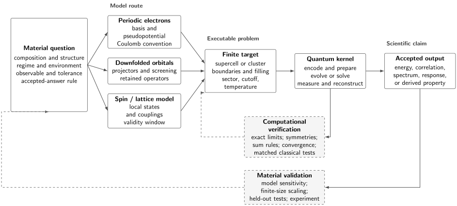
Three legitimate starting points lead to different approximation ledgers. Periodic electronic structure, a downfolded active-orbital model, or an effective spin or lattice Hamiltonian must first become a convention-complete finite target. Encoding, preparation, evolution or solving, and measurement form the quantum kernel. Acceptance requires both computational verification and an observable-level return to classical calculations and material data.

Three Hamiltonian Routes

Periodic electronic structure

For fixed nuclei in a periodic cell, an all-electron starting point has the form

$$\begin{aligned} H_{\mathrm e} ={}& \sum_{i=1}^{\eta} \left[ -\frac{\hbar^2}{2m_{\mathrm e}}\nabla_i^2 + V_{\mathrm{ion}}(\mathbf r_i) \right] \\ &+ \frac12 \sum_{i\ne j} \frac{e^2}{ 4\pi\epsilon_0 \lvert\mathbf r_i-\mathbf r_j\rvert } + E_{\mathrm{ion}}. \end{aligned}$$

The actual computational Hamiltonian may replace core electrons by pseudopotentials, represent orbitals in plane waves, real-space grids, atomic functions, or Wannier functions, and evaluate long-range Coulomb terms with a periodic convention. Each choice changes both physical approximation error and quantum resources.

Periodic first-principles simulation is not just molecular simulation with a larger atom count. It introduces a thermodynamic sequence, reciprocal-space sampling, charged-cell conventions, extensive energies, and often many closely spaced states. The primitive cell can be small while the correlated many-electron problem remains hard.

Downfolded orbital Hamiltonians

A lower-energy description retains selected localized orbitals $w_{ia}(\mathbf r)$, where $i$ labels a cell or correlated site and $a$ an orbital. A general static form is

$$\begin{aligned} H_{\mathrm{eff}} ={}& E_0 + \sum_{ij} \sum_{ab} \sum_{\sigma\sigma'} t_{ij}^{ab,\sigma\sigma'} c_{ia\sigma}^{\dagger} c_{jb\sigma'} \\ &+ \frac12 \sum_{ijkl} \sum_{abcd} \sum_{\sigma\sigma'} U_{ijkl}^{abcd} c_{ia\sigma}^{\dagger} c_{jb\sigma'}^{\dagger} c_{ld\sigma'} c_{kc\sigma} + \cdots . \end{aligned}$$

The ellipsis matters. Projection can generate longer-range hopping, exchange, pair hopping, correlated hopping, retarded interactions, and higher-body operators. Dropping them is a model approximation, not a free simplification performed by the encoder.

If $P$ projects onto the active subspace and $Q=I-P$, exact elimination is formally energy dependent:

$$H_{\mathrm{eff}}(E) = PHP + PHQ \frac{1}{E-QHQ} QHP.$$

A static Hubbard-family Hamiltonian therefore requires a scale-separation or fitting argument. The page on Effective Hamiltonians in Quantum Matter develops this logic, while Hubbard Physics in Materials handles orbital windows, screened interactions, and double counting.

Spin, boson, and phenomenological models

When local moments or collective modes are already justified, the input can be a spin, rotor, boson, or constrained lattice Hamiltonian. A general bilinear spin model is

$$H_{\mathrm{spin}} = \sum_{i<j} \sum_{\alpha,\beta} J_{ij}^{\alpha\beta} S_i^\alpha S_j^\beta - \sum_i \mathbf h_i\cdot\mathbf S_i + H_{\mathrm{multi}}.$$

$H_{\mathrm{multi}}$ can include single-ion anisotropy, ring exchange, or other multi-spin terms. The exchange tensor, spin length, local axes, graph, boundary conditions, and validity window are part of the model. Replacing an itinerant or charge-transfer material by a rigid-spin model requires evidence; the visual resemblance of an ordered phase is not enough.

Route	Natural strengths	Material-specific risks
periodic electrons	ab initio energies, forces, charge and quasiparticle questions	basis and pseudopotential error, Coulomb finite size, state preparation
downfolded orbitals	strong local correlations in a smaller active space	projector dependence, screening, double counting, omitted operators
spin or lattice model	compact local Hilbert space and native analog realizations	uncertain parameter map, missing charge/orbital channels, restricted validity

Finite Periodic Targets

Supercell and boundary data

A processor always receives a finite problem. For a supercell containing $N_{\mathrm c}$ primitive cells, report its shape, lattice vectors, number of active modes per cell, particle sector, and treatment of long-range terms. Two clusters with the same site count can have different coordination, frustration, allowed momenta, and low-energy spectra.

Twisted boundary conditions in direction $\alpha$ take the form

$$\Psi( \ldots, \mathbf r_i+L_\alpha\mathbf a_\alpha, \ldots ) = e^{i\theta_\alpha} \Psi( \ldots, \mathbf r_i, \ldots ).$$

For a one-dimensional length-$L$ ring, the allowed momenta are

$$k_n = \frac{2\pi n+\theta}{L}.$$

Changing $\boldsymbol\theta$ shifts the finite momentum grid without changing the bulk Hamiltonian. Twist averaging,

$$\overline O_L = \frac{1}{M_\theta} \sum_{m=1}^{M_\theta} O_L(\boldsymbol\theta_m),$$

can reduce shell effects, but it does not remove interaction finite-size errors, correlation-length effects, or an incorrect thermodynamic extrapolation. Boundary conventions are especially important after a fermionic mapping, where parity and physical twists must not be conflated.

Intensive and nonextensive precision

If a bulk ground-state energy is

$$E(N_{\mathrm c}) = N_{\mathrm c}e_\infty + \delta E_{\mathrm{fs}},$$

then estimating the energy density to error $\delta e$ permits total-energy error of order $N_{\mathrm c}\delta e$, before finite-size extrapolation. This is why a resource estimate for energy per cell can scale differently from one for a fixed absolute energy.

Many useful outputs do not receive that relaxation:

• an excitation gap is an $O(1)$ energy difference;
• a defect or adsorption energy subtracts two extensive calculations;
• a phase competition may depend on a small energy difference per cell;
• a response peak can require resolution much finer than the total bandwidth.

The requested observable, not the phrase “ground-state energy,” sets the precision target.

Thermodynamic and critical limits

A finite cluster cannot by itself establish a bulk phase. Near a continuous transition, the correlation length can become comparable with every available linear size. One then needs a declared finite-size scaling ansatz, aspect-ratio control, boundary tests, and enough sizes to distinguish scaling corrections from the leading behavior. The Finite-Size Scaling in Numerics page owns the full methodology.

From Material Degrees of Freedom to Qubits

Spin and qudit sites

A spin-$1/2$ site maps directly to one qubit when

$$S_i^\alpha = \frac12\sigma_i^\alpha.$$

The factor $1/2$ must be propagated into every coupling. A spin-$S$ site has dimension $2S+1$ and can use a binary, unary, or hardware-native qudit encoding. Binary encodings use fewer qubits, while unary or qudit encodings can make local operators simpler. Leakage and unused binary states require an explicit detection or penalty strategy.

Fermionic modes

In a Jordan–Wigner convention with $n_j=(I-Z_j)/2$,

$$c_j = \left( \prod_{k<j} Z_k \right) \frac{X_j+iY_j}{2}.$$

One spin orbital uses one qubit, but geometric locality need not survive. A nearest-neighbor hop on a two-dimensional lattice can become a long Pauli string after the sites are ordered along a line. Fermionic swaps, parity or Bravyi–Kitaev-type encodings, and locality-preserving mappings trade string length against auxiliary qubits, stabilizer constraints, and circuit complexity.

A mapping is therefore specified by more than its qubit count:

1. fermionic mode order;
2. Pauli convention and occupation eigenvalue;
3. boundary and parity sector;
4. auxiliary or gauge constraints;
5. routing strategy on the hardware graph;
6. the mapped forms of all measured observables.

An encoding that localizes the Hamiltonian but makes the target Green function or string order parameter expensive may be the wrong choice.

Bosonic and collective modes

A bosonic site must be truncated, for example to

$$n_i \in \{0,1,\ldots,n_{\max}\}.$$

A compact binary register needs

$$q_i = \left\lceil \log_2(n_{\max}+1) \right\rceil$$

qubits, with unused states when $n_{\max}+1$ is not a power of two. Convergence requires increasing $n_{\max}$ and checking the target observable. Merely observing little probability at the highest retained occupation is useful but not universally sufficient, because virtual occupation near the cutoff can renormalize low-energy quantities.

Symmetry reduction

Particle number, spin projection, translation, point-group quantum numbers, and discrete parities can reduce the relevant state space. Exact tapering is valid only when the encoded Hamiltonian commutes with the symmetry and the desired state lies in the chosen sector. Penalty terms are not the same as eliminating a degree of freedom: they change spectral scales and can introduce optimization or simulation costs.

Momentum-space encodings can expose translation symmetry while making local interactions dense. Real-space encodings preserve sparse locality while hiding momentum labels. The resource comparison must include the complete Hamiltonian, state preparation, routing, and observable map in the same basis.

State Preparation Is a Materials Bottleneck

Ground states and low-lying states

Common starting states include noninteracting Fermi seas, mean-field Slater determinants, tensor-network states, product-ordered states, and states prepared at an easier parameter point. None guarantees useful overlap in a strongly correlated regime.

If phase estimation begins in

$$\lvert\psi_{\mathrm{in}}\rangle = \sum_k a_k\lvert E_k\rangle,$$

then the target eigenvalue is obtained with ideal probability

$$p_0 = \lvert a_0\rvert^2.$$

After $r$ independent attempts, the probability of seeing it at least once is

$$P_{\mathrm{hit}} = 1-(1-p_0)^r.$$

The overlap can therefore dominate a favorable Hamiltonian-simulation query count. It must be estimated or bounded for the stated system-size sequence, not inferred from one small cluster.

Adiabatic continuation uses

$$H(s) = (1-s)H_0+sH_1, \qquad 0\le s\le1.$$

Its cost depends on the minimum relevant gap, transition matrix elements, and schedule along the path. Small gaps near symmetry changes or phase transitions can erase the apparent simplicity of preparing the endpoint. Changing the path can help, but only if it preserves the intended final sector and does not replace the target problem.

Finite systems and broken symmetry

A finite Hamiltonian that respects a symmetry can have a symmetric ground state even when the thermodynamic phase breaks that symmetry. Thus $\langle M\rangle=0$ on a finite cluster does not rule out order. A typical diagnostic is a structure factor

$$S_O(\mathbf q) = \frac{1}{N} \sum_{ij} e^{i\mathbf q\cdot(\mathbf r_i-\mathbf r_j)} \langle O_i O_j\rangle.$$

Long-range order is inferred from the size dependence of $S_O(\mathbf Q)/N$, susceptibility, gaps, and boundary or pinning-field responses. Preparing one symmetry-broken branch can be physically useful, but the preparation protocol and order of limits must be stated.

Thermal states

Finite-temperature material properties require

$$\rho_\beta = \frac{e^{-\beta H}}{Z}, \qquad Z = \operatorname{Tr}e^{-\beta H},$$

or another explicitly defined nonequilibrium ensemble. Ground-state algorithms do not solve this task by changing a label. Gibbs-state preparation can involve purification, imaginary-time or variational methods, rejection steps, or engineered open dynamics, and its cost can worsen at low temperature, across phase transitions, or with unfavorable free-energy differences.

Uncontrolled hardware noise is not a thermal bath at a known temperature. Calling a noisy output “finite-temperature physics” requires a calibrated effective channel and independent thermodynamic checks.

Choosing the Quantum Route

Route	Best-matched task	Dominant limitation to report
analog simulator	native spin, Hubbard, or bosonic dynamics and snapshots	Hamiltonian calibration, restricted terms, temperature, observable map
variational digital method	approximate low-energy states on shallower circuits	ansatz bias, optimization, shots, noise, scaling evidence
digitized adiabatic preparation	connection from an accessible state	minimum gap, schedule, coherent depth
phase estimation	systematic eigenvalues on fault-tolerant hardware	input overlap, controlled evolution, absolute precision
real-time simulation	quenches, transport kernels, spectra, response	state preparation, maximum time, time step, repeated measurements
embedding with a quantum kernel	correlated impurity or active cluster in a classical loop	bath discretization, self-consistency, kernel noise, outer-loop stability

VQE owns variational bounds, measurement allocation, optimization, and ansatz error. Quantum Phase Estimation owns phase statistics and resolution. Hamiltonian Simulation compares evolution oracles and costs, Trotter–Suzuki Methods owns product-formula error, and Qubitization and Quantum Signal Processing owns block encodings, normalization, signal processing, and query expansion. This page asks which of those tools returns the specified materials observable.

Representation Controls Algorithmic Cost

The same electronic problem can look very different in different bases. Localized orbitals often make hopping and interactions spatially sparse but can require many orbitals per cell and carefully screened interaction tensors. Plane waves give systematic kinetic-energy cutoffs and efficient basis changes, while Coulomb operators and pseudopotentials have their own data-access and normalization costs. A dual plane-wave representation can diagonalize different Hamiltonian pieces in complementary bases, making basis transforms part of each simulation step.

For a Pauli decomposition

$$H_q = \sum_{\ell=1}^{L} h_\ell P_\ell, \qquad \lambda = \sum_{\ell=1}^{L} \lvert h_\ell\rvert,$$

neither the mode count nor $L$ alone determines cost. Product formulas depend on commutators, ordering, target time, and observable. LCU and qubitization depend on the block-encoding normalization and the cost of preparing and selecting terms. Hardware execution adds routing, synthesis, error correction, and repeated state preparation.

Materials often offer structure that should be exploited:

• translation-related terms can share coefficients and control logic;
• low-rank interaction factorizations can reduce data and arithmetic;
• local spin Hamiltonians can be edge colored for parallel layers;
• Fourier transforms can alternate diagonal kinetic and potential pieces;
• symmetries can reduce sectors or provide verification checks.

Every simplification must preserve the finite target and the requested observable. A resource claim should include the circuit that loads coefficients or performs arithmetic, not assume the Hamiltonian appears as a free oracle.

Embedding and Self-Consistent Workflows

A quantum processor need not represent the whole crystal. In dynamical mean-field and related embedding approaches, a classical outer loop maps a lattice problem to a correlated impurity or cluster coupled to an effective bath. A quantum kernel may prepare the impurity state or estimate its Green function, after which the classical loop updates the bath and repeats.

This changes the resource question. The total cost includes

$$N_{\mathrm{kernel}} = N_{\mathrm{outer}} N_{\mathrm{frequency}} N_{\mathrm{parameter}} N_{\mathrm{repeat}},$$

up to opportunities for reusing data or measuring several frequencies together. Bath discretization, self-consistency tolerance, causal Green functions, and convergence from distinct initial guesses remain mandatory. A small impurity register is not automatically a cheap material calculation.

Embedding can be scientifically powerful because it concentrates quantum resources on a strongly correlated subspace while classical methods handle the environment. It is also vulnerable to mismatched approximations: a precise impurity solver cannot repair an inadequate embedding functional, active space, or double-counting convention.

Observables, Not Wavefunctions, Are the Output

Energies and derived properties

Bulk energy densities, phase differences, formation energies, voltages, forces, stresses, and migration barriers use different combinations of energies. For example, a defect formation energy schematically has the form

$$E_{\mathrm f} = E_{\mathrm{defect}} - E_{\mathrm{bulk}} - \sum_a n_a\mu_a + E_{\mathrm{corr}}.$$

The two extensive energies must use compatible cells, basis conventions, boundary corrections, and accuracy. Chemical potentials and finite-size corrections belong to the answer. An accurate isolated energy does not certify the cancellation.

Correlations and scattering observables

Equal-time correlations diagnose order, entanglement, and characteristic wavevectors. Dynamical probes require two-time correlators such as

$$C_A(\mathbf q,t) = \langle A_{\mathbf q}(t) A_{-\mathbf q}(0) \rangle,$$

and a spectral transform

$$S_A(\mathbf q,\omega) = \frac{1}{2\pi} \int_{-\infty}^{\infty} dt\, e^{i\omega t} C_A(\mathbf q,t).$$

A finite time window $\lvert t\rvert\le T$ broadens spectral features on an energy scale of order $2\pi\hbar/T$. Discrete sampling limits the accessible bandwidth, while windows trade resolution and sidelobes. Noise, mitigation, and Fourier processing create correlated uncertainties across frequencies. The Structure Factors page owns the scattering conventions.

Single-particle spectra

Photoemission-like information is related to the retarded Green function

$$G_{pq}^{R}(t) = -i\Theta(t) \left\langle \left\{ c_p(t), c_q^\dagger(0) \right\} \right\rangle,$$

with spectral function

$$A_{pq}(\omega) = -\frac{1}{\pi} \operatorname{Im} G_{pq}^{R}(\omega).$$

This output involves particle-addition and particle-removal sectors, phase coherence, real-time evolution or spectral sampling, and frequency reconstruction. A ground-state energy algorithm does not provide it for free. Spectral Functions owns Lehmann representations, sum rules, and interpretation.

Response and transport

Conductivity, susceptibility, and other response coefficients require the appropriate current or generalized-force operators, contact or diamagnetic terms when present, a state or ensemble, and an order of limits in frequency, wavevector, size, and broadening. The Kubo Formula owns the response derivation. A quantum routine that estimates one current correlator still needs the complete observable convention and extrapolation.

Worked Encoding Audit: The Hubbard Dimer

The two-site repulsive Hubbard model is too small to establish a material phase, but it is an excellent convention and observable audit:

$$\begin{aligned} H ={}& -t \sum_{\sigma} \left( c_{1\sigma}^{\dagger}c_{2\sigma} + c_{2\sigma}^{\dagger}c_{1\sigma} \right) \\ &+ U \sum_{i=1}^{2} n_{i\uparrow}n_{i\downarrow}. \end{aligned}$$

Order the modes as

$$\left( 1\uparrow,\, 2\uparrow,\, 1\downarrow,\, 2\downarrow \right) \longleftrightarrow \left( q_0,q_1,q_2,q_3 \right).$$

Jordan–Wigner then gives

$$\begin{aligned} H_q ={}& -\frac{t}{2} \left( X_0X_1+Y_0Y_1 + X_2X_3+Y_2Y_3 \right) \\ &+ \frac{U}{4} \left[ (I-Z_0)(I-Z_2) + (I-Z_1)(I-Z_3) \right]. \end{aligned}$$

This ordering makes hopping adjacent but places each onsite interaction across the two spin registers. Site-major ordering does the opposite: onsite terms become adjacent while hopping acquires parity strings. The spectrum is unchanged under a consistent remapping, but native depth need not be.

At half filling the full fixed-particle sector has dimension

$$\binom{4}{2} = 6,$$

far below the full $2^4=16$ qubit space. In the symmetry block containing the ground state, choose phases so that the covalent singlet $\lvert C\rangle$ and symmetric doublon state $\lvert D_+\rangle$ give

$$H_{\mathrm{block}} = \begin{pmatrix} 0 & -2t\\ -2t & U \end{pmatrix}.$$

The ground energy is

$$E_0 = \frac{ U-\sqrt{U^2+16t^2} }{2}.$$

The Hellmann–Feynman theorem turns an energy derivative into total double occupation:

$$\begin{aligned} D &= \left\langle \sum_i n_{i\uparrow}n_{i\downarrow} \right\rangle \\ &= \frac{\partial E_0}{\partial U} = \frac12 \left( 1- \frac{U}{\sqrt{U^2+16t^2}} \right). \end{aligned}$$

For $U\gg\lvert t\rvert$,

$$E_0 = -\frac{4t^2}{U} + O\!\left( \frac{t^4}{U^3} \right), \qquad D = \frac{4t^2}{U^2} + O\!\left( \frac{t^4}{U^4} \right).$$

The triplet energy is zero in this convention, so the singlet–triplet splitting approaches $4t^2/U$. A valid implementation should reproduce the $U=0$ bonding energy, particle and spin symmetries, these strong-coupling limits, and the derivative relation before it is trusted on larger lattices. The Hubbard Model and its model dossiers own the fuller physics.

A Layered Error Ledger

Let $O_{\mathrm{mat}}$ be the intended material quantity, $O_{\mathrm{model}}$ the exact prediction of the chosen effective model, $O_L$ the exact finite-instance result, $O_{\mathrm{enc}}$ the exact result of the encoded and truncated Hamiltonian, and $\widehat O$ the reported estimate. A diagnostic decomposition is

$$\begin{aligned} \widehat O-O_{\mathrm{mat}} ={}& \left( O_{\mathrm{model}}-O_{\mathrm{mat}} \right) + \left( O_L-O_{\mathrm{model}} \right) \\ &+ \left( O_{\mathrm{enc}}-O_L \right) + \left( \widehat O-O_{\mathrm{enc}} \right). \end{aligned}$$

The four terms collect:

1. material-model error: structure, active subspace, screened parameters, phonons, disorder, environment, and omitted interactions;
2. finite-instance error: cell size and shape, boundaries, momentum or twist sampling, temperature grid, and thermodynamic extrapolation;
3. encoding error: basis cutoff, boson truncation, coefficient precision, pseudopotentials, auxiliary constraints, and symmetry reduction;
4. solution and inference error: state preparation, evolution or variational bias, hardware noise, mitigation, sampling, transforms, fitting, and derived-property propagation.

This additive expression is bookkeeping, not a promise that uncertainties are independent or worst-case bounds are tight. Correlated errors, cancellation, and nonlinear postprocessing require covariance or sensitivity analysis. The important discipline is that device accuracy cannot erase material-model error.

Resource Accounting

A reproducible estimate should report at least:

Layer	Quantities to record
physical target	cells, orbitals or local states, filling, boundaries, temperature, observable
Hamiltonian data	term count, coefficient precision, sparsity or factorization, norm or block-encoding normalization
logical registers	system, symmetry, index, arithmetic, phase, and work qubits
preparation	circuit, overlap or fidelity target, success probability, retries
quantum kernel	oracle calls, Trotter steps or QSP degree, logical gates, depth, routing
output	measurement settings, shots, maximum time, frequency grid, confidence
fault tolerance	code and decoder assumptions, code distance, factories, physical qubits, runtime
workflow multiplicity	structures, twists, fillings, temperatures, frequencies, outer iterations
classical work	model construction, compilation, optimization, postprocessing, extrapolation, validation

The last two rows are easy to hide. A battery voltage, phase boundary, or spectral map may require hundreds of related quantum calls even when one Hamiltonian instance is affordable. Warm starts and correlated sampling can reduce cost, but they must be demonstrated rather than assumed.

Resource Estimation Tools owns logical-to-physical compilation and uncertainty sweeps.

Verification and Material Validation

Verify the finite computation

Before leaving the classically accessible regime:

1. compare mapped and unmapped spectra on tiny instances;
2. recover noninteracting, atomic, decoupled, or exactly solvable limits;
3. test Hermiticity, conserved charges, stabilizers, and boundary conventions;
4. verify energy derivatives against independently measured observables;
5. test step size, ansatz depth, basis cutoff, coefficient precision, and measurement allocation;
6. check spectral sum rules and causal or positivity constraints;
7. compare several initial states and symmetry sectors;
8. blind at least one parameter point or observable during calibration.

Validate the model

Computational correctness asks whether the processor solved the declared finite Hamiltonian. Material validity asks whether that Hamiltonian answers the physical question. The latter needs:

• convergence under plausible orbital windows, supercells, and omitted terms;
• agreement with several independent observables, not only fitted targets;
• transfer across temperature, pressure, filling, or momentum when claimed;
• comparison with competing model families;
• uncertainty propagated to the final material property;
• clear weakening or rejection of the model when held-out evidence fails.

Use a portfolio of classical baselines

The strongest classical comparator depends on regime. Exact diagonalization is decisive for small clusters. Tensor networks can dominate low-entanglement one-dimensional and quasi-one-dimensional problems. Quantum Monte Carlo can scale well in sign-problem-free regions. Perturbation theory, coupled cluster, embedding, dynamical mean-field methods, and specialized free-fermion or integrability techniques each have favorable domains.

A fair comparison fixes the Hamiltonian, cell and boundaries, state, observable, tolerance, confidence, and included pre- and postprocessing. A quantum–classical disagreement is a diagnostic, not proof that the quantum answer is correct. Algorithmic Benchmarking owns accepted-answer rules and matched time-to-solution comparisons.

Common Mistakes

• Calling an abstract lattice-model calculation a prediction for a material.
• Treating a fitted Hubbard $U$ or exchange $J$ as basis-independent.
• Reporting a site count without orbitals, spin modes, filling, and boundary conditions.
• Assuming a small primitive cell implies a small correlated problem.
• Ignoring parity strings, routing, or auxiliary constraints in fermionic encodings.
• Comparing qubit count while omitting Hamiltonian data access and coefficient precision.
• Treating a finite symmetric state with zero order parameter as evidence against thermodynamic symmetry breaking.
• Calling uncontrolled device noise a thermal ensemble.
• Reporting only ground-state energy when the material question concerns a spectrum, response, defect, force, or phase boundary.
• Using energy-per-cell precision for an $O(1)$ gap or defect energy.
• Comparing with a generic classical method rather than the best matched regime-specific portfolio.
• Validating the solver and assuming that this validates the material model.
• Extrapolating one cluster, one parameter point, or one observable into a phase diagram.
• Calling a logical query count an end-to-end resource estimate.

Reporting Checklist

A materials-simulation result should make it possible to answer:

1. What material, model, regime, and observable are claimed?
2. Is the goal mechanism discovery, effective-model solution, or property prediction?
3. How were the active degrees of freedom and parameters obtained?
4. What finite cell, geometry, boundary, filling, and symmetry sector were used?
5. What encoding, mode order, truncations, and coefficient precision were used?
6. How was the state or ensemble prepared, and what is the success criterion?
7. Which quantum solver and error controls were used?
8. How was the observable reconstructed, including all repeated preparations?
9. How were finite-size, basis, model, hardware, and statistical errors propagated?
10. Which classical methods and experimental data were used for verification and held-out validation?
11. What logical, physical, classical, and workflow-wide resources are included?
12. What narrower conclusion remains if the strongest interpretation fails?

Research Status

As of August 2026, quantum processors and analog simulators have produced scientifically informative results for finite Hubbard, Ising, Heisenberg, and related many-body models. The strongest demonstrations combine calibrated Hamiltonians, exact small-instance checks, symmetry or sum-rule tests, observable-level error analysis, and serious classical comparison.

Near-term digital calculations remain constrained by preparation depth, sampling, optimization, routing, and noise. Analog platforms can access larger native arrays, but model calibration, restricted interactions, temperature, and extrapolation limit material claims. Quantum Green-function, embedding, and thermal-state methods are active research areas with small demonstrations and developing complexity results.

Fault-tolerant studies provide valuable algorithms and resource estimates for periodic electrons and correlated lattice models. They are projections whose conclusions depend on representation, state overlap, precision, architecture, and the number of material instances. No broadly accepted end-to-end practical advantage for predicting a useful real-material property has yet been established. This does not erase the scientific value of model experiments or the possibility of future advantage; it sets the evidence threshold.

References

1. R. P. Feynman, “Simulating Physics with Computers,” International Journal of Theoretical Physics 21, 467–488 (1982).
2. I. M. Georgescu, S. Ashhab, and F. Nori, “Quantum Simulation,” Reviews of Modern Physics 86, 153–185 (2014).
3. B. Bauer, S. Bravyi, M. Motta, and G. K.-L. Chan, “Quantum Algorithms for Quantum Chemistry and Quantum Materials Science,” Chemical Reviews 120, 12685–12717 (2020).
4. E. Altman et al., “Quantum Simulators: Architectures and Opportunities,” PRX Quantum 2, 017003 (2021).
5. R. Babbush, N. Wiebe, J. McClean, J. McClain, H. Neven, and G. K.-L. Chan, “Low-Depth Quantum Simulation of Materials,” Physical Review X 8, 011044 (2018).
6. I. D. Kivlichan et al., “Improved Fault-Tolerant Quantum Simulation of Condensed-Phase Correlated Electrons via Trotterization,” Quantum 4, 296 (2020).
7. C. Cade, L. Mineh, A. Montanaro, and S. Stanisic, “Strategies for Solving the Fermi–Hubbard Model on Near-Term Quantum Computers,” Physical Review B 102, 235122 (2020).
8. S. Stanisic et al., “Observing Ground-State Properties of the Fermi–Hubbard Model Using a Scalable Algorithm on a Quantum Computer,” Nature Communications 13, 5743 (2022).
9. D. Wecker, M. B. Hastings, and M. Troyer, “Progress towards Practical Quantum Variational Algorithms,” Physical Review A 92, 042303 (2015).
10. S. Bravyi and A. Kitaev, “Fermionic Quantum Computation,” Annals of Physics 298, 210–226 (2002).
11. J. D. Whitfield, V. Havlíček, and M. Troyer, “Local Spin Operators for Fermion Simulations,” Physical Review A 94, 030301(R) (2016).
12. Y.-A. Chen and Y. Xu, “Equivalence between Fermion-to-Qubit Mappings in Two Spatial Dimensions,” PRX Quantum 4, 010326 (2023).
13. J. Rizzo, F. Libbi, F. Tacchino, P. J. Ollitrault, N. Marzari, and I. Tavernelli, “One-Particle Green’s Functions from the Quantum Equation of Motion Algorithm,” Physical Review Research 4, 043011 (2022).
14. P. Rall, C. Wang, and P. Wocjan, “Thermal State Preparation via Rounding Promises,” Quantum 7, 1132 (2023).
15. A. Georges, G. Kotliar, W. Krauth, and M. J. Rozenberg, “Dynamical Mean-Field Theory of Strongly Correlated Fermion Systems and the Limit of Infinite Dimensions,” Reviews of Modern Physics 68, 13–125 (1996).
16. S. R. White, “Density Matrix Formulation for Quantum Renormalization Groups,” Physical Review Letters 69, 2863–2866 (1992).
17. C. Lin, F. H. Zong, and D. M. Ceperley, “Twist-Averaged Boundary Conditions in Continuum Quantum Monte Carlo Algorithms,” Physical Review E 64, 016702 (2001).
18. N. Marzari, A. A. Mostofi, J. R. Yates, I. Souza, and D. Vanderbilt, “Maximally Localized Wannier Functions: Theory and Applications,” Reviews of Modern Physics 84, 1419–1475 (2012).
19. M. Imada and T. Miyake, “Electronic Structure Calculation by First Principles for Strongly Correlated Electron Systems,” Journal of the Physical Society of Japan 79, 112001 (2010).
20. A. Delgado et al., “Simulating Key Properties of Lithium-Ion Batteries with a Fault-Tolerant Quantum Computer,” Physical Review A 106, 032428 (2022).
21. A. W. Daley et al., “Practical Quantum Advantage in Quantum Simulation,” Nature 607, 667–676 (2022).

Further Connections

• Materials Simulation Case Studies assesses cold-atom Hubbard experiments, Rydberg and kicked-Ising studies, direct material comparisons, and fault-tolerant projections.
• Band Theory Overview supplies the crystalline one-electron language from which periodic and downfolded models begin.
• Hubbard Model owns operator conventions, symmetries, exact limits, and generic diagnostics.
• Heisenberg Model owns isotropic spin exchange and its finite-system physics.
• Dynamical Correlation Functions Numerically develops time-window, frequency-resolution, and reconstruction issues for classical and quantum workflows.
• Benchmark Problems identifies convention-complete finite targets for cross-method validation.

Exercises

1. Complete a materials contract

A proposal says: “Use 100 qubits to simulate a cuprate Hubbard model and measure superconductivity.” List at least six pieces of missing information needed to make this a reproducible computational claim.

Solution

A sufficient answer should include at least:

1. the active orbitals and whether the model is one-band, three-band, or another downfolding;
2. the lattice geometry, cluster shape, and boundary conditions;
3. hopping, interaction, chemical-potential, and longer-range terms with units and sign conventions;
4. the filling or particle-number sector;
5. the state or temperature and its preparation protocol;
6. the superconducting observable, such as a pair correlation, susceptibility, stiffness, or response to a pairing field;
7. the finite-size scaling or accepted finite-instance claim;
8. the fermionic encoding, mode order, qubit meaning, and symmetry reduction;
9. the solver, error budget, shots, and confidence;
10. the classical and experimental validation data.

“Measure superconductivity” is not yet an observable. On a finite number-conserving cluster, a one-point anomalous expectation can vanish even when pair correlations are strong, so the order-of-limits and diagnostic matter.

2. Derive the twisted momentum grid

For a one-dimensional ring of length $L$, impose $\psi(x+L)=e^{i\theta}\psi(x)$. Derive the allowed plane-wave momenta and state the periodic and antiperiodic special cases.

Solution

For $\psi_k(x)=e^{ikx}$, the boundary condition gives

$$e^{ik(x+L)} = e^{i\theta}e^{ikx},$$

so

$$kL = \theta+2\pi n, \qquad k_n = \frac{2\pi n+\theta}{L}, \quad n\in\mathbb Z.$$

$\theta=0$ gives periodic momenta $2\pi n/L$. $\theta=\pi$ gives antiperiodic momenta $2\pi(n+1/2)/L$. Averaging several twists samples shifted finite momentum grids, but it does not by itself perform an interacting thermodynamic extrapolation.

3. Count modes and a symmetry sector

An eight-site spinful Hubbard cluster uses one qubit per fermionic mode. How many qubits are required? At half filling with $N_\uparrow=N_\downarrow=4$, what is the dimension of that fixed-spin-number sector? Compare it with the full qubit Hilbert space.

Solution

Each site has an up and down spin orbital, so there are

$$N_{\mathrm{mode}} = 2L = 16$$

modes and therefore 16 qubits in a direct occupation encoding. The fixed sector has dimension

$$\dim\mathcal H_{4,4} = \binom{8}{4} \binom{8}{4} = 70^2 = 4900.$$

The full qubit Hilbert space has dimension

$$2^{16} = 65536.$$

Symmetry-aware preparation and simulation can avoid much of the unused space, although the physical qubit register need not shrink unless the encoding explicitly compresses or tapers it.

4. Check the Hubbard-dimer limits

Starting from

$$E_0 = \frac{ U-\sqrt{U^2+16t^2} }{2},$$

find $E_0$ and total double occupation $D=\partial E_0/\partial U$ at $U=0$. Then obtain their leading large-$U$ behavior.

Solution

At $U=0$,

$$E_0 = -2\lvert t\rvert.$$

For the convention $t>0$, this is $-2t$. Differentiating gives

$$D = \frac12 \left( 1- \frac{U}{\sqrt{U^2+16t^2}} \right),$$

so $D(0)=1/2$. This is the total probability of double occupation across the two sites for two electrons in the bonding orbital.

For $U\gg\lvert t\rvert$,

$$\sqrt{U^2+16t^2} = U \left( 1+\frac{8t^2}{U^2} -\frac{32t^4}{U^4} +\cdots \right).$$

Therefore

$$E_0 = -\frac{4t^2}{U} + \frac{16t^4}{U^3} + \cdots,$$

and

$$D = \frac{4t^2}{U^2} - \frac{48t^4}{U^4} + \cdots.$$

Both limits are useful implementation tests.

5. Distinguish bulk and defect precision

A 100-cell calculation targets a bulk energy density to $1\,\mathrm{meV}$ per cell. What total-energy error is compatible with that target before finite-size extrapolation? Why can the same tolerance not be used for a defect formation energy required to $10\,\mathrm{meV}$?

Solution

For the bulk energy density,

$$\delta E = N_{\mathrm c}\delta e = 100\times1\,\mathrm{meV} = 0.1\,\mathrm{eV}.$$

The defect formation energy is an $O(1)$ difference between extensive quantities. Allowing each total energy an uncontrolled $0.1\,\mathrm{eV}$ error could overwhelm a $10\,\mathrm{meV}$ target. The bulk and defect calculations need compatible conventions and a joint error allocation at the few-meV scale, depending on covariance and the other chemical-potential and correction terms. Extensive cancellation does not make the required absolute precision disappear.

6. Budget overlap-dependent repetitions

A state-preparation protocol has target overlap probability $p_0=0.08$. How many independent phase-estimation attempts are required so that the target is seen at least once with probability at least $0.99$?

Solution

Require

$$1-(1-p_0)^r \ge 0.99.$$

Thus

$$r \ge \frac{\ln(0.01)}{\ln(0.92)} \approx 55.23.$$

The first integer that guarantees the target is therefore

$$r=56.$$

This count precedes failures from imperfect controlled evolution, readout, or target-eigenvalue identification.

7. Relate evolution time to spectral resolution

Using the order-of-magnitude relation $\Delta E\sim2\pi\hbar/T$, estimate the time window needed to resolve two spectral features separated by $5\,\mathrm{meV}$. Use $2\pi\hbar\approx4.136\,\mathrm{eV\,fs}$.

Solution

The required time is

$$T \sim \frac{2\pi\hbar}{\Delta E} = \frac{ 4.136\,\mathrm{eV\,fs} }{ 0.005\,\mathrm{eV} } \approx 827\,\mathrm{fs}.$$

Thus the coherent or reconstructed correlation window is of order $0.83\,\mathrm{ps}$. Windowing and a desired confidence can require a longer record. The sampling interval separately controls the largest resolvable frequency.

8. Diagnose an overstrong material claim

A quantum device reproduces the exact energy and double occupation of a $2\times4$ Hubbard cluster at one value of $U/t$. The authors conclude that a named bulk oxide is a one-band Hubbard material and that its phase diagram has been computed. Separate what the result verifies from what remains unproved.

Solution

Agreement verifies, within the stated uncertainty, that the device and postprocessing reproduced two observables of that finite Hamiltonian at one parameter point. It is valuable evidence for encoding, preparation, measurement, and solver behavior.

It does not establish:

• that the oxide reduces to a one-band model;
• that the chosen hopping and $U$ follow from a valid orbital and screening construction;
• that omitted ligand, orbital, phonon, spin–orbit, disorder, or longer-range terms are negligible;
• that the cluster represents the thermodynamic limit;
• that two observables determine a phase;
• that behavior transfers across filling, temperature, pressure, or $U/t$;
• that the best classical methods cannot answer the same question.

The material claim needs model validation against independent probes and plausible alternative models. The phase-diagram claim needs multiple parameters, sizes, diagnostics, and controlled extrapolation.