What Is Quantum Simulation?

Definition and Scope

A quantum simulation uses controllable quantum degrees of freedom to infer a property of a specified target quantum model. The target may represent a molecule, a lattice magnet, an interacting field, a driven open system, or an abstract Hamiltonian. The simulator may be a programmable quantum computer, a purpose-built many-body experiment, or a hybrid quantum–classical system.

The definition has three essential parts:

1. A target question: a quantity, state property, dynamical response, sample distribution, or decision to be obtained.
2. A model correspondence: an explicit map between target degrees of freedom and the simulator.
3. A trust argument: evidence and bounds connecting measured simulator data to the target answer.

Merely evolving a quantum device is not yet a simulation. The device becomes a simulator only after the target model, mapping, observables, operating regime, and uncertainty are declared. Conversely, a useful simulator need not reproduce every microscopic feature of a real material. It may faithfully answer one well-defined question about an idealized model.

This page is the canonical home for that simulation contract, the digital–analog–hybrid taxonomy, error accounting, and the interpretation of simulation claims. Verification of Quantum Simulation develops the evidence architecture for hard regimes. Lattice Models Overview owns the physics of common target models. Hamiltonian Simulation owns the simulation-facing Hamiltonian task, access-instance, error, output, and method-selection contract. Trotter Product Formula owns product-formula derivations. Ultracold-Atom Quantum Simulation owns a platform-specific frontier assessment.

Materials Simulation Case Studies compares complete Hubbard, spin-model, material-validation, and fault-tolerant-property claims without duplicating the simulation contract.

The Simulation Contract

For a closed-system dynamical task, specify a target Hilbert space $\mathcal H_{\mathrm{tar}}$, an initial state $\rho_{\mathrm{tar}}(0)$, a Hamiltonian $H_{\mathrm{tar}}$, and observables $O_\alpha$. The ideal target prediction is

$$\mu_\alpha(t) = \operatorname{Tr} \left[ O_\alpha U_{\mathrm{tar}}(t) \rho_{\mathrm{tar}}(0) U_{\mathrm{tar}}^\dagger(t) \right],$$

with

$$U_{\mathrm{tar}}(t) = e^{-iH_{\mathrm{tar}}t/\hbar}.$$

A simulator supplies an encoding into its controllable degrees of freedom, implements approximate dynamics, and measures data from which $\mu_\alpha(t)$ is estimated. A mature statement therefore declares:

Contract item	Required specification
scientific question	target quantity and why it answers the physical question
target model	Hilbert space, Hamiltonian or channel, parameters, boundaries, and approximations
regime	sizes, times, energies, couplings, temperatures, and parameter domain
representation	qubit, qudit, bosonic, fermionic, gauge, or effective-subspace encoding
state preparation	input state, thermal ensemble, quench protocol, or ground-state method
implemented dynamics	gate sequence, pulse schedule, engineered Hamiltonian, or dissipative process
measurement	observables, basis rotations, detector model, and number of shots
inference	estimator, reconstruction, extrapolation, and uncertainty statement
resources	qubits or modes, gates, evolution time, energy, repetitions, and classical computation
validation	solvable limits, convergence tests, calibrated generators, symmetries, and independent checks

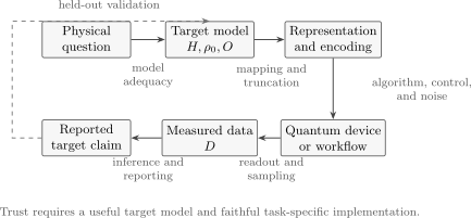
A simulation claim crosses several interfaces. Model adequacy connects a physical system to an idealized target model; implementation fidelity connects that model to the encoded device and its data. Validation must test both, because precise execution of an inadequate model and imprecise execution of a good model are different failures.

Two distinct links must be trusted

Suppose a real system of interest is represented by a model $M$, and a device implements an approximation $\widetilde M$. Two questions follow:

1. Model validation: does $M$ describe the real system in the claimed regime?
2. Simulator verification: does the device implement $M$ accurately enough for the declared observable?

These questions do not collapse into one fidelity number. A quantum computer can simulate an ideal lattice Hamiltonian very accurately even if that Hamiltonian is a poor model of a material. An analog experiment can reproduce a qualitative phase pattern while its couplings differ enough from the target to invalidate a quantitative critical point. Scientific interpretation requires both links.

The distinction also clarifies why simulation can be valuable when it rejects a model. If a verified simulator predicts behavior inconsistent with experiment, the target model may be incomplete. The simulator has still produced useful evidence.

What a Quantum Simulator Returns

A simulator does not normally return the full many-body wavefunction. It returns task-specific classical information extracted from repeated measurements, such as:

• an energy or spectral gap;
• a local density, magnetization, current, or order parameter;
• an equal-time or dynamical correlation function;
• samples from a many-body distribution;
• a response to a quench, ramp, pulse, or external field;
• a phase boundary or critical exponent with finite-size qualifications;
• a prepared state for use by another quantum procedure;
• a decision between competing models.

For example, a two-point correlation function may be

$$C_{ij}^{zz}(t) = \operatorname{Tr} \left[ Z_iZ_j\rho(t) \right] - \operatorname{Tr} \left[ Z_i\rho(t) \right] \operatorname{Tr} \left[ Z_j\rho(t) \right].$$

The ability to prepare $\rho(t)$ does not grant free access to all of its amplitudes or all observables. Each incompatible measurement setting consumes additional preparations, and full tomography generally scales poorly with system size. Output and measurement cost belong in the problem definition, not in a footnote after the evolution has been implemented.

Why Use a Quantum Device?

For $n$ distinguishable subsystems of local dimension $d$, a generic pure state requires $d^n$ complex amplitudes in a product basis. This exponential state-space growth motivates quantum simulation: a physical quantum system represents its state without storing a classical list of every amplitude.

That observation is important but is not a complexity proof. Many quantum models are classically tractable because of integrability, weak correlations, free-particle structure, stabilizer structure, low entanglement, favorable Monte Carlo weights, or a restricted observable and time regime. Conversely, hard state preparation, long coherent evolution, or expensive readout can remove an apparent quantum benefit.

Lloyd’s universal-simulation result established efficient digital simulation for broad classes of local quantum systems under explicit locality and accuracy assumptions. It does not imply that every quantum-model question is efficiently solvable. Ground-state preparation may be hard, evolution time can itself be a resource, and extracting a tiny signal can require many repetitions.

A defensible motivation therefore has this form:

For the stated family of inputs, target observable, error tolerance, and access model, the quantum device has a plausible end-to-end resource advantage over the best applicable classical methods.

“The Hilbert space is exponentially large” and “a Monte Carlo method has a sign problem” are warning signs of possible classical difficulty, not stand-alone demonstrations of quantum advantage.

Digital Quantum Simulation

A digital quantum simulator encodes the target degrees of freedom into registers and approximates the desired operation with a sequence of discrete gates. If $V:\mathcal H_{\mathrm{tar}}\to\mathcal H_{\mathrm{sim}}$ is an isometric encoding and $W(t)$ is the implemented circuit, a natural logical-space requirement is

$$\left\| V^\dagger W(t)V - U_{\mathrm{tar}}(t) \right\| \le \epsilon_{\mathrm{sim}}.$$

The norm and domain must be stated. Operator norm controls every encoded input state, while a state- or observable-specific guarantee may be much weaker and cheaper.

When

$$H_{\mathrm{tar}} = \sum_{\ell=1}^{L} H_\ell,$$

one route is a product formula. For two bounded terms and $\Delta t=t/r$,

$$e^{-i(H_A+H_B)t/\hbar} \approx \left( e^{-iH_A\Delta t/\hbar} e^{-iH_B\Delta t/\hbar} \right)^r.$$

The leading first-order error is controlled by noncommutativity and scales schematically as

$$\epsilon_{\mathrm{PF}} = O\!\left( \frac{t^2}{r\hbar^2} \left\| [H_A,H_B] \right\| \right),$$

subject to the bounded-operator assumptions behind the estimate. Higher-order product formulas, linear-combination methods, truncated Taylor series, qubitization, and quantum signal processing provide other tradeoffs. Their detailed algorithmic complexity belongs on dedicated pages.

Digital simulation offers a common gate-level interface, programmable model changes, and systematic algorithmic error parameters. Those benefits do not make it automatically accurate. Compilation, synthesis, control, crosstalk, leakage, decoherence, logical error correction, state preparation, and measurement each contribute additional error and cost.

Analog Quantum Simulation

An analog quantum simulator engineers a device Hamiltonian whose behavior corresponds directly to a target family. A useful abstract mapping is

$$P H_{\mathrm{lab}} P = \alpha V H_{\mathrm{tar}} V^\dagger + \beta P + \Delta H,$$

where:

• $P$ projects onto the intended simulator subspace;
• $V$ maps target states into that subspace;
• $\alpha$ fixes the energy and time scale;
• $\beta$ contributes only a global phase for closed dynamics within $P$;
• $\Delta H$ contains unwanted couplings, inhomogeneity, truncation, and calibration error.

If $\Delta H=0$, target time $t$ corresponds to laboratory time $t/\alpha$. The observable must also be mapped: a detector reading $O_{\mathrm{lab}}$ answers the target question only when its relation to $V O_{\mathrm{tar}}V^\dagger$ is controlled.

Analog devices can realize large, continuously evolving systems with fewer compiled operations than a gate-by-gate construction. They can also expose local correlations and nonequilibrium dynamics naturally. Their central difficulty is that the implemented generator is physical rather than symbolic. Long-range tails, trap inhomogeneity, residual levels, finite temperature, loss, and imperfect constraints are part of the actual model.

An analog simulator is therefore not validated by a visual resemblance between two phase diagrams. It needs a quantitative mapping, parameter calibration, regime statement, and observable-level uncertainty.

Hybrid Quantum Simulation

Hybrid simulation combines distinct quantum and classical roles. The label includes at least three different patterns:

1. Digital–analog simulation: native many-body blocks provide analog evolution, while discrete gates and pulses reconfigure or compose those blocks.
2. Variational simulation: a parameterized quantum state or process is measured, and a classical optimizer updates the parameters.
3. Quantum embedding: a quantum device treats a selected correlated subsystem while a classical method supplies an environment, mean field, or self-consistency loop.

The word hybrid is not an error model. A complete description must say which object is represented quantum mechanically, which quantities cross the classical interface, how the loop terminates, and how uncertainty and optimizer failure are handled.

Hybrid Quantum Simulation develops these three interface architectures, including native-block composition, tangent-space projection, self-consistent embedding, feedback stability, and end-to-end resource accounting.

Variational energy estimation, for example, evaluates

$$E(\boldsymbol\theta) = \langle\psi(\boldsymbol\theta)| H |\psi(\boldsymbol\theta)\rangle$$

on a quantum device and updates $\boldsymbol\theta$ classically. The method is only as useful as its ansatz expressivity, optimization landscape, measurement allocation, noise sensitivity, and comparison with classical variational states.

Emulator, Simulator, and Universal Computer

Terminology is not perfectly uniform, so capability should be described directly.

Term	Typical meaning	What it does not guarantee
quantum emulator	specialized device reproducing a restricted model family or phenomenon	quantitative accuracy outside the calibrated regime
analog simulator	engineered continuous Hamiltonian or channel with a direct target correspondence	universality or a tunable error parameter
digital simulator	gate-based algorithm approximating target dynamics	low physical overhead or useful output extraction
universal quantum computer	programmable device able, in principle, to approximate arbitrary quantum circuits	that a particular simulation is efficient, verified, or scientifically useful
hybrid simulator	quantum process embedded in digital–analog or quantum–classical workflow	convergence, advantage, or immunity to classical bottlenecks

A universal computer can act as a digital simulator. A specialized analog device can be scientifically valuable without being universal. “Emulation” often emphasizes a restricted correspondence, but it should not be used to evade an error budget.

The Error Budget

Simulation errors arise at different conceptual layers:

$$\begin{aligned} \epsilon_{\mathrm{total}} \;\text{depends on}\;& \epsilon_{\mathrm{model}}, \epsilon_{\mathrm{map}}, \epsilon_{\mathrm{prep}}, \epsilon_{\mathrm{dyn}}, \\ & \epsilon_{\mathrm{noise}}, \epsilon_{\mathrm{readout}}, \epsilon_{\mathrm{stat}}, \epsilon_{\mathrm{infer}}. \end{aligned}$$

These symbols need not be directly additive. Some are norms, some are confidence bounds, and some are model-discrepancy assessments. They should be propagated to the reported quantity in compatible units.

State and observable error

If $\rho$ is the ideal target state, $\widetilde\rho$ is the effective simulator state in the same representation, and

$$D(\rho,\widetilde\rho) = \frac{1}{2} \left\| \rho-\widetilde\rho \right\|_1,$$

then any bounded observable obeys

$$\left| \operatorname{Tr} \left[ O(\rho-\widetilde\rho) \right] \right| \le 2 \left\|O\right\|_\infty D(\rho,\widetilde\rho).$$

This converts a state-distance statement into a worst-case observable bound. It may be far more conservative than a task-specific estimate, but it makes the dependence explicit.

For channels, a diamond-norm bound can control errors uniformly over inputs, including entangled reference systems. In practice, full channel characterization is expensive, so local generators, selected observables, and structured error models are often tested instead.

Algorithmic and physical errors are different

Increasing the product-formula step count can reduce ideal discretization error while increasing circuit depth and physical noise. A schematic observable error might behave as

$$\epsilon_{\mathrm{obs}}(r) \lesssim \frac{A}{r^p} + B r + \epsilon_0,$$

where $A/r^p$ is algorithmic error, $Br$ is accumulated hardware error, and $\epsilon_0$ collects preparation and readout floors. The optimal finite $r$ is not the formal limit $r\to\infty$.

For an analog device, the corresponding control parameter may be evolution time, detuning, interaction range, or protection strength. Error can grow nonlinearly near resonances, critical points, unstable dynamics, or leakage thresholds.

Finite sampling is part of the algorithm

Suppose a measured observable has outcomes in $[-1,1]$ and sample mean $\widehat\mu$. Hoeffding’s inequality gives

$$\Pr \left( \left| \widehat\mu-\mu \right| \ge \epsilon \right) \le 2e^{-N\epsilon^2/2}.$$

Thus a sufficient shot count for failure probability at most $\delta$ is

$$N \ge \frac{2}{\epsilon^2} \ln \frac{2}{\delta}.$$

This cost must be multiplied by parameter points, time points, measurement bases, and mitigation variants. An evolution circuit that is efficient in gate complexity can still have an expensive measurement layer.

Open-System Simulation

The target need not be unitary. A Markovian open-system target may obey

$$\frac{d\rho}{dt} = -\frac{i}{\hbar}[H,\rho] + \sum_\mu \gamma_\mu \left( L_\mu\rho L_\mu^\dagger - \frac{1}{2} \left\{ L_\mu^\dagger L_\mu,\rho \right\} \right).$$

This dynamics can be simulated through ancillas and gates, stochastic unravelings, collision models, or engineered dissipation. Lindblad–GKSL Equation owns the formal generator and its assumptions.

Uncontrolled hardware decoherence is not automatically a faithful simulation of target dissipation. The noise operators, rates, correlations, initial system–environment conditions, and Markov approximations must match the declared open-system model. “The device is noisy, so it naturally simulates an open system” is usually too weak to support a quantitative claim.

Worked Example: Transverse-Field Ising Dynamics

Consider the open-chain target

$$H_{\mathrm{tar}} = -J \sum_{j=1}^{n-1} Z_jZ_{j+1} - h \sum_{j=1}^{n} X_j.$$

Prepare $\lvert0\rangle^{\otimes n}$, quench to nonzero $J$ and $h$, and ask for

$$m_z(t) = \frac{1}{n} \sum_{j=1}^{n} \langle Z_j(t)\rangle$$

and selected connected correlations $C_{ij}^{zz}(t)$. This is already a complete task only after $n$, boundaries, parameter ranges, time grid, precision, and confidence level are fixed.

Digital realization

With $\Delta t=t/r$, a first-order circuit is

$$\begin{aligned} W_r(t) = \Bigg[ & \prod_{j=1}^{n-1} e^{\,iJ\Delta t Z_jZ_{j+1}/\hbar} \\ &\times \prod_{j=1}^{n} e^{\,ih\Delta t X_j/\hbar} \Bigg]^r. \end{aligned}$$

The two-body terms commute with one another, as do the one-body terms, but the two groups do not commute. Varying $r$ tests product-formula convergence until physical gate errors dominate. The Transverse-Field Ising Model page owns the model’s many-body physics.

Analog realization

An analog platform may implement

$$H_{\mathrm{lab}} = - \sum_{i<j} J_{ij}Z_iZ_j - \sum_i h_iX_i + H_{\mathrm{res}}.$$

To claim nearest-neighbor Ising simulation, the measured $J_{ij}$, field inhomogeneity $h_i-h$, residual term $H_{\mathrm{res}}$, boundary conditions, and time rescaling must be included. Long-range interactions are not merely “noise” if they materially change the model; the honest target may instead be a long-range Ising model.

Validation ladder

The same task admits several checks:

1. At $J=0$, each spin undergoes an independent rotation and

   $$m_z(t) = \cos \left( \frac{2ht}{\hbar} \right).$$

2. At $h=0$, $\lvert0\rangle^{\otimes n}$ is an eigenstate, so $m_z(t)=1$.

3. Small systems can be compared with exact diagonalization.

4. Digital results should converge over a range of $r$ before hardware noise reverses the trend.

5. The global spin-flip symmetry $\prod_j X_j$ commutes with the ideal Hamiltonian and can expose certain implementation errors.

6. Independently calibrated couplings can be used to make held-out predictions at times or parameters not used in fitting.

No single check proves correctness everywhere. Together they establish a ladder from analytically controlled limits toward the classically difficult regime.

Verification and Validation

Verification should be designed around the intended output. Full tomography of a large simulator is usually unnecessary and infeasible; testing the relevant generator, symmetries, and observables can be more informative.

Method	What it tests	Main limitation
exact small-size comparison	end-to-end agreement where classical calculation is reliable	may not expose errors that grow with size
short-time expansion	local generator moments and early dynamics	does not validate long-time behavior
solvable limits	parameter dependence and known asymptotes	errors may appear away from the limit
conservation laws and constraints	leakage, symmetry breaking, gauge violation, or drift	passing necessary conditions is not sufficient
convergence tests	Trotter step, truncation, size, bond dimension, or measurement allocation	hardware and algorithmic errors can trade off
Hamiltonian or channel learning	implemented generator and parameter uncertainty	depends on model identifiability
cross-platform comparison	consistency between independent implementations	shared theory and analysis assumptions can correlate errors
randomized measurements	overlaps, purities, correlations, and cross-device state comparisons	sample and control demands can be substantial
blind or held-out prediction	extrapolative power beyond calibration data	requires disciplined separation of fitting and testing

Calibration data should not be recycled as decisive validation data without disclosure. A model with enough fitted parameters can agree with the observations used to construct it. Held-out controls, times, initial states, or observables test whether the correspondence predicts rather than merely describes.

Resource Accounting and Advantage Claims

At least three claims are often conflated:

1. Classically challenging operation: the device reaches a regime that is difficult for a named classical method.
2. Computational quantum advantage: the quantum workflow solves the same formal input–output task at the same error with better scaling or resources than the best applicable classical workflow.
3. Scientific utility: the simulation produces reliable insight, prediction, or model discrimination that matters for science.

None implies the other two automatically. A classically difficult sample distribution may answer no useful physical question. A scientifically valuable analog simulator may not have a proved asymptotic advantage. A formal algorithmic speedup may require fault-tolerant resources beyond the experiment being discussed.

A comparison should count:

• target size, parameter domain, and requested observable;
• error tolerance and success probability;
• state preparation and equilibration time;
• logical gates, analog evolution, or coherent interrogation time;
• repetitions and measurement settings;
• calibration, mitigation, and discarded runs;
• classical compilation, optimization, inference, and verification;
• hardware parallelism and energy only when compared on a common boundary;
• the strongest classical algorithm available for the same structured instance.

The Claims, Hype, and Evidence Standards page supplies the broader vocabulary for separating theorem, algorithm, resource estimate, demonstration, benchmark, and application.

Common Mistakes

Treating a large Hilbert space as a speedup proof

Exponential state-space dimension motivates the field but does not identify the complexity of a particular input–output task.

Calling every controlled quantum experiment a simulation

The target model, mapping, observable, and trust argument must be explicit.

Confusing target-model error with device error

A perfect simulator of an inadequate model can make a precise but physically irrelevant prediction.

Relabeling unwanted noise as open-system physics

Target dissipation has specified operators, rates, correlations, and approximations. Uncharacterized decoherence does not satisfy that contract.

Reporting only state or gate fidelity

The scientifically relevant quantity may be a correlation, phase boundary, rare-event probability, or response coefficient whose error behaves differently.

Ignoring state preparation and readout

Efficient time evolution does not imply efficient ground-state preparation, thermalization, amplitude extraction, or tomography.

Comparing against a weak classical baseline

Exact diagonalization is not the only classical method. Tensor networks, Monte Carlo, perturbation theory, embedding, symmetries, and problem-specific approximations may change the comparison.

Treating a sign problem as a universal impossibility theorem

A sign problem obstructs a chosen Monte Carlo representation. It does not rule out every classical algorithm for every observable and instance.

Using agreement at one point as global validation

Error sensitivity can change with size, time, coupling, phase, and observable. Extrapolation needs its own evidence.

Equating universality with usefulness

A universal device may be too costly for the task, while a special-purpose simulator may answer it efficiently and reliably.

Exercises

1. Identify the simulation contract

An experiment prepares 50 ions, applies a tunable interaction for $5\,\mathrm{ms}$, and plots spin correlations. List six pieces of information still needed before the plot constitutes a quantum-simulation result.

Solution

Possible required items are: the target Hamiltonian or channel; the map from ion levels to target spins; the initial state; the calibrated interaction graph and field strengths; the target time corresponding to $5\,\mathrm{ms}$; the measured correlation definition; the detector and readout model; statistical uncertainty; unwanted couplings and decoherence; the parameter regime; and validation tests. Any six that cover the target, mapping, operation, output, and uncertainty expose why “controlled ions plus a plot” is incomplete.

2. Classify three simulators

Classify each workflow as digital, analog, or hybrid:

1. a gate circuit applies product-formula steps for a molecular Hamiltonian;
2. atoms in an optical lattice realize a Bose–Hubbard Hamiltonian directly;
3. a parameterized circuit measures an energy and a classical optimizer updates its angles.

Solution

The first is digital because a discrete gate sequence approximates target evolution. The second is analog because an engineered physical Hamiltonian directly realizes the target model over a calibrated regime. The third is hybrid because quantum state preparation and measurement are embedded in a classical optimization loop. The labels do not establish accuracy; each workflow still needs its own mapping and error budget.

3. Show why the analog energy offset is harmless

Assume

$$P H_{\mathrm{lab}}P = \alpha V H_{\mathrm{tar}}V^\dagger + \beta P$$

with no leakage. Show that $\beta$ does not affect expectation values of encoded observables.

Solution

Within the encoded subspace,

$$e^{-iH_{\mathrm{lab}}t_{\mathrm{lab}}/\hbar} = e^{-i\beta t_{\mathrm{lab}}/\hbar} V e^{-iH_{\mathrm{tar}}t/\hbar} V^\dagger,$$

where $t=\alpha t_{\mathrm{lab}}$. The first factor is a global phase. It cancels between the ket and bra in a density operator and therefore cancels from

$$\operatorname{Tr} \left[ V O V^\dagger \rho_{\mathrm{lab}}(t_{\mathrm{lab}}) \right].$$

The offset is harmless only while evolution remains within $P$; subspace-dependent offsets or leakage need not be.

4. Recover the product-formula error scaling

Use the Baker–Campbell–Hausdorff expansion to explain why repeating

$$e^{-iH_A\Delta t/\hbar} e^{-iH_B\Delta t/\hbar}$$

for $r=t/\Delta t$ steps gives a leading global error proportional to $t^2\lVert[H_A,H_B]\rVert/(r\hbar^2)$.

Solution

Let $A=-iH_A\Delta t/\hbar$ and $B=-iH_B\Delta t/\hbar$. The Baker–Campbell–Hausdorff expansion gives

$$e^Ae^B = \exp \left( A+B+\frac{1}{2}[A,B]+O(\Delta t^3) \right).$$

Because

$$[A,B] = -\frac{\Delta t^2}{\hbar^2} [H_A,H_B],$$

the local error is $O(\Delta t^2\lVert[H_A,H_B]\rVert/\hbar^2)$. Accumulating $r$ steps gives the schematic global scale

$$r\Delta t^2 \frac{\lVert[H_A,H_B]\rVert}{\hbar^2} = \frac{t^2}{r} \frac{\lVert[H_A,H_B]\rVert}{\hbar^2}.$$

Rigorous constants and long-time growth require the assumptions developed on the product-formula page.

5. Solve two Ising validation limits

For the worked Ising example with initial state $\lvert0\rangle^{\otimes n}$, find $m_z(t)$ when (a) $J=0$ and (b) $h=0$.

Solution

When $J=0$, each spin evolves under $-hX$. The single-spin unitary is

$$e^{\,ihtX/\hbar},$$

which rotates the Bloch vector about the $x$ axis by angle $2ht/\hbar$. Therefore

$$m_z(t) = \cos \left( \frac{2ht}{\hbar} \right).$$

When $h=0$, the initial computational-basis state is an eigenstate of every $Z_jZ_{j+1}$ term. Evolution adds only a phase, so every $\langle Z_j\rangle=1$ and $m_z(t)=1$.

6. Convert trace distance to observable error

Suppose $D(\rho,\widetilde\rho)\le0.015$ and $\lVert O\rVert_\infty=1$. What worst-case bias in $\langle O\rangle$ follows from the trace-distance bound?

Solution

Using

$$\left| \operatorname{Tr} \left[ O(\rho-\widetilde\rho) \right] \right| \le 2\lVert O\rVert_\infty D(\rho,\widetilde\rho),$$

the bias is at most

$$2(1)(0.015)=0.030.$$

This is a uniform worst-case bound. Knowledge of the observable and error structure may yield a tighter task-specific estimate.

7. Budget the number of shots

For outcomes in $[-1,1]$, use Hoeffding’s inequality to find a sufficient $N$ for additive error $\epsilon=0.02$ and failure probability $\delta=0.01$.

Solution

The sufficient condition is

$$N \ge \frac{2}{\epsilon^2} \ln \frac{2}{\delta}.$$

Substitution gives

$$\begin{aligned} N &\ge \frac{2}{0.02^2} \ln(200) \\ &\approx 5000(5.298) \\ &\approx 26492. \end{aligned}$$

Thus $N=26492$ shots suffice after rounding up. This conservative bound applies per independently estimated bounded observable and setting.

8. Find the optimal digital step count

Suppose a simplified error model is

$$\epsilon(r) = \frac{0.8}{r} + 0.002r + 0.01.$$

Treating $r$ as continuous, find the minimizing step count and explain why $r\to\infty$ is not optimal.

Solution

Differentiate:

$$\frac{d\epsilon}{dr} = -\frac{0.8}{r^2} + 0.002.$$

Setting this to zero gives

$$r^2 = \frac{0.8}{0.002} = 400, \qquad r=20.$$

The product-formula term decreases with $r$, but hardware error grows with circuit depth. The constant $0.01$ floor does not affect the optimum. An integer search around $r=20$ would complete the practical choice.

9. Design a held-out validation test

An analog simulator’s couplings are fitted using magnetization traces from three initial states up to time $t_0$. Propose a held-out test that checks predictive power rather than fit quality.

Solution

Freeze the fitted model and predict data not used in calibration: for example, a connected two-point correlation from a fourth initial state at times between $t_0$ and $1.5t_0$. Predeclare the observable, time window, uncertainty band, and acceptance criterion. The new state tests preparation dependence, the correlation tests more than the fitted one-body observable, and the later times test accumulated generator error. Re-fitting after seeing the held-out data would turn the test back into calibration and should be reported separately.

10. Audit an advantage claim

A paper states: “Our 100-qubit analog simulator has quantum advantage because exact diagonalization would require $2^{100}$ amplitudes.” Give four reasons this does not yet establish computational quantum advantage.

Solution

First, exact diagonalization is not necessarily the strongest classical method; tensor networks, Monte Carlo, symmetries, or specialized approximations may apply. Second, the input–output task and accuracy are unspecified, so the compared computations are not defined. Third, state preparation, repetitions, readout, calibration, and classical postprocessing are omitted from the quantum resource count. Fourth, the result has not been verified in the claimed regime. A serious advantage claim also needs scaling over a problem family and a matched classical baseline, not only one Hilbert-space dimension.

References

1. R. P. Feynman, “Simulating physics with computers,” International Journal of Theoretical Physics 21, 467–488 (1982), doi:10.1007/BF02650179.
2. S. Lloyd, “Universal quantum simulators,” Science 273, 1073–1078 (1996), doi:10.1126/science.273.5278.1073.
3. I. Buluta and F. Nori, “Quantum simulators,” Science 326, 108–111 (2009), doi:10.1126/science.1177838.
4. J. I. Cirac and P. Zoller, “Goals and opportunities in quantum simulation,” Nature Physics 8, 264–266 (2012), doi:10.1038/nphys2275.
5. I. M. Georgescu, S. Ashhab, and F. Nori, “Quantum simulation,” Reviews of Modern Physics 86, 153–185 (2014), doi:10.1103/RevModPhys.86.153.
6. T. H. Johnson, S. R. Clark, and D. Jaksch, “What is a quantum simulator?” EPJ Quantum Technology 1, 10 (2014), doi:10.1140/epjqt10.
7. E. Altman et al., “Quantum simulators: Architectures and opportunities,” PRX Quantum 2, 017003 (2021), doi:10.1103/PRXQuantum.2.017003.
8. P. Hauke, F. M. Cucchietti, L. Tagliacozzo, I. H. Deutsch, and M. Lewenstein, “Can one trust quantum simulators?” Reports on Progress in Physics 75, 082401 (2012), doi:10.1088/0034-4885/75/8/082401.
9. J. Eisert et al., “Quantum certification and benchmarking,” Nature Reviews Physics 2, 382–390 (2020), doi:10.1038/s42254-020-0186-4.
10. J. Carrasco, A. Elben, C. Kokail, B. Kraus, and P. Zoller, “Theoretical and experimental perspectives of quantum verification,” PRX Quantum 2, 010102 (2021), doi:10.1103/PRXQuantum.2.010102.
11. I. Bloch, J. Dalibard, and S. Nascimbène, “Quantum simulations with ultracold quantum gases,” Nature Physics 8, 267–276 (2012), doi:10.1038/nphys2259.
12. R. Blatt and C. F. Roos, “Quantum simulations with trapped ions,” Nature Physics 8, 277–284 (2012), doi:10.1038/nphys2252.
13. A. A. Houck, H. E. Türeci, and J. Koch, “On-chip quantum simulation with superconducting circuits,” Nature Physics 8, 292–299 (2012), doi:10.1038/nphys2251.
14. D. W. Berry, A. M. Childs, R. Cleve, R. Kothari, and R. D. Somma, “Simulating Hamiltonian dynamics with a truncated Taylor series,” Physical Review Letters 114, 090502 (2015), doi:10.1103/PhysRevLett.114.090502.
15. G. H. Low and I. L. Chuang, “Optimal Hamiltonian simulation by quantum signal processing,” Physical Review Letters 118, 010501 (2017), doi:10.1103/PhysRevLett.118.010501.
16. S. P. Jordan, K. S. M. Lee, and J. Preskill, “Quantum algorithms for quantum field theories,” Science 336, 1130–1133 (2012), doi:10.1126/science.1217069.
17. F. Schäfer et al., “Tools for quantum simulation with ultracold atoms in optical lattices,” Nature Reviews Physics 2, 411–425 (2020), doi:10.1038/s42254-020-0195-3.

Further Connections

• Quantum Information and Computation places simulation beside computation, communication, and sensing as a distinct input–output task.
• Digital Quantum Simulation develops the encoded-Hamiltonian, gate-compilation, observable-estimation, resource, and error-accounting workflow for digital implementations.
• Analog Quantum Simulation develops the target–device Hamiltonian correspondence, effective-model reduction, control manifold, observable error, and validation workflow for native many-body dynamics.
• Quantum Circuit Simulation covers classical execution of gate-model circuits; it is distinct from using a quantum device to emulate a physical target model.
• What Is Quantum Information? introduces the shared preparation–channel–measurement language.
• Algorithmic Primitives explains how Hamiltonian access, block encoding, product formulas, and quantum signal processing compose with other algorithms.
• Trotter Product Formula derives the operator splitting, while Trotter–Suzuki Methods develops its simulation-level error scaling, resources, and validation.
• Lattice Models Overview and Quantum Matter own the target many-body and materials physics.
• Computational Many-Body Overview maps the classical methods that belong in a serious baseline comparison.
• Ultracold-Atom Quantum Simulation provides a dated evidence ledger for optical-lattice and atom-array simulators.
• Quantum Channels and Noise supplies channel metrics for noisy and open-system implementations.
• Quantum Information Roadmap places simulation after states, measurements, circuits, algorithms, and noise.