Superconducting Quantum Simulators

Short Definition

A superconducting quantum simulator uses quantized electrical circuits at microwave frequencies to reproduce selected quantum states, dynamics, spectra, response functions, or steady states. Its simulated degrees of freedom may be two-level subspaces of artificial atoms, weakly anharmonic oscillators, resonator photons, light–matter polaritons, or deliberately encoded logical variables.

Three implementation families recur:

1. qubit lattices, in which artificial atoms represent spins or hard-core bosons;
2. resonator and polariton arrays, in which microwave modes realize itinerant bosons with engineered hopping, interactions, drive, and loss;
3. programmable circuit networks, in which tunable or parametrically driven couplers synthesize interactions, complex hopping phases, and digital–analog schedules.

These families overlap physically. A transmon is itself a weakly anharmonic oscillator, and the same chip may be described as a qubit processor in one experiment and as a Bose–Hubbard lattice in another. The scientific claim is therefore fixed by the controlled subspace, generator, preparation, observable, and error budget, not by the device label.

Canonical Scope

This page is the canonical home for the map from a superconducting circuit to a quantum-simulation claim. It develops:

• the reduction from circuit modes to qubits, bosons, or polaritons;
• the distinction among qubit lattices, resonator arrays, and driven-coupler networks;
• native analog, digital, digital–analog, and open-system routes;
• platform-specific preparation, readout, calibration, and resource costs;
• leakage, parasitic interactions, drive dressing, decoherence, and drift;
• evidence needed to support a result about a target model.

The underlying implementation physics has other canonical homes. Circuit QED Overview derives circuit modes, artificial atoms, resonator coupling, dispersive readout, and microwave control. Superconducting Qubits owns qubit families, processor architecture, packaging, noise, and scaling. Open-System Circuit QED owns measurement backaction, master equations, and trajectories. Generic analog, digital, hybrid, and open-system simulation workflows remain canonical on their respective pages.

The question here is narrower and more operational:

Given a target model and requested observable, what circuit was actually implemented, what reduction connects it to the target, and what evidence bounds the discrepancy?

The Simulation Contract

A reproducible superconducting simulation should specify a contract

$$\mathcal C = \left( \mathcal H_{\mathrm{tar}}, \mathcal G_{\mathrm{tar}}, \rho_0, \mathcal P, O, \epsilon, \mathcal E \right),$$

where:

• $\mathcal H_{\mathrm{tar}}$ is the target Hilbert space or constrained state space;
• $\mathcal G_{\mathrm{tar}}$ is the Hamiltonian, channel, or open-system generator;
• $\rho_0$ is the intended initial state or state-preparation rule;
• $\mathcal P$ is the schedule of quenches, ramps, drives, gates, or dissipative stages;
• $O$ is the observable or estimator returned by the experiment;
• $\epsilon$ is the requested accuracy, resolution, or hypothesis-test threshold;
• $\mathcal E$ is the evidence used to validate the correspondence.

The device supplies a physical Hilbert space $\mathcal H_{\mathrm{dev}}$, a generator $\mathcal G_{\mathrm{dev}}(\lambda)$ controlled by calibrated parameters $\lambda$, and a measurement instrument $\mathcal M$. An encoding or model reduction $V$ must connect the target and device descriptions. For a closed-system Hamiltonian target, the central obligation is not merely $\dim \mathcal H_{\mathrm{dev}}\geq\dim \mathcal H_{\mathrm{tar}}$. It is a controlled statement of the form

$$V^\dagger H_{\mathrm{dev}}(\lambda)V = H_{\mathrm{tar}} + \Delta H,$$

together with a bound or empirical characterization of $\Delta H$ on the states, time window, and observables actually used.

For open-system targets, the analogous statement concerns generators or channels,

$$V^\dagger \mathcal L_{\mathrm{dev}}(lambda) V = \mathcal L_{\mathrm{tar}} + \Delta\mathcal L.$$

Here the notation is schematic: a subspace restriction of a quantum channel must preserve complete positivity and account for leakage. A projection that silently discards leaked population is not automatically a physical reduced channel.

Why Superconducting Circuits Are Distinct

Superconducting circuits combine five properties that shape their use as simulators.

They are fabricated Hamiltonians. Capacitances, inductances, Josephson energies, resonator geometry, and coupling networks set much of the bare model. Fabrication makes unusual graphs and nonlinearities possible, but it also introduces device-to-device disorder that cannot be tuned away in every architecture.

Their parameters are fast and local. Microwave drives and flux controls can change frequencies, couplings, phases, and measurement bases on nanosecond-to-microsecond scales. This supports quenches, echoes, Floquet engineering, and digital–analog protocols.

Their excitations need not obey a natural conservation law. Microwave photons may be injected and removed coherently or dissipatively. This makes driven nonequilibrium matter especially natural, while making an equilibrium chemical potential nontrivial.

Their measurement is strong and information rich. Multiplexed dispersive readout can return site-resolved bitstrings; resonator output can return complex field quadratures and spectra. Yet readout resonators, amplifiers, filters, and classifiers form a measurement instrument with its own error model.

Their coherence is finite and control dependent. Relaxation and dephasing coexist with leakage, flux noise, residual $ZZ$ interactions, microwave crosstalk, coupler excitations, and calibration drift. A simulator may deliberately engineer dissipation, but uncontrolled loss does not thereby become target physics.

Platform Map

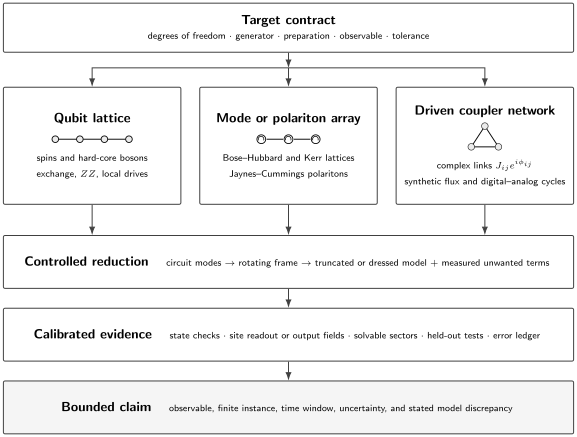
A superconducting simulation is a chain of models. Qubit lattices, nonlinear mode arrays, and driven-coupler networks are distinct reductions of a circuit, not interchangeable labels. Calibration and readout must support the final claim about the target observable.

Circuit realization	Effective variables	Natural model families	Characteristic obligations
Qubit lattice	two-level sites, hard-core excitations	$XY$, Ising, Heisenberg-type, quantum walks	leakage, residual couplings, rotating-frame calibration
Nonlinear resonator array	bosonic occupations	Bose–Hubbard, Kerr lattices, driven fluids of light	Fock-space cutoff, photon loss, drive calibration
Qubit–resonator array	polaritons	Jaynes–Cummings–Hubbard and related light–matter lattices	branch identification, occupation-dependent interaction
Parametric coupler network	spins or bosons with complex links	synthetic gauge fields, Floquet and topological models	phase conventions, micromotion, unwanted sidebands
Gate-programmable processor	encoded qubits or qudits	broad digital model classes	compilation, gate error, depth, sampling

No row is universally superior. The useful realization is the one whose native degrees of freedom, preparation, observables, and dominant errors fit the scientific question.

From Circuit Hamiltonian to Target Model

The most important derivation is usually not the final many-body calculation. It is the sequence of approximations connecting the fabricated circuit to the implemented model:

$$\begin{gathered} \text{electromagnetic circuit} \longrightarrow \text{quantized normal modes} \longrightarrow \text{weakly nonlinear mode model} \\ \longrightarrow \text{rotating-frame effective Hamiltonian} \longrightarrow \text{encoded target model}. \end{gathered}$$

Each arrow has a domain of validity. Common steps include linear-mode diagonalization, expansion of Josephson nonlinearities, truncation of local Hilbert spaces, a rotating-wave approximation, perturbative elimination of off-resonant modes, Floquet averaging, and projection onto a computational or polariton manifold.

The full derivation should preserve enough of the microscopic model to estimate omitted terms. A target Hamiltonian written from symmetry alone does not reveal whether the device also contains next-nearest-neighbor hopping, cross-Kerr interactions, correlated drive terms, frequency-dependent loss, or coupling to a package mode.

A useful hierarchy of models

For a weakly anharmonic network, a common intermediate description is

$$\begin{aligned} \frac{H_{\mathrm{mode}}}{\hbar} ={}& \sum_i \left[ \omega_i n_i + \frac{\alpha_i}{2}n_i(n_i-1) \right] \\ &+ \sum_{i<j} \left( J_{ij}a_i^\dagger a_j + J_{ij}^*a_j^\dagger a_i \right) + H_{\mathrm{parasitic}} + H_{\mathrm{drive}}(t), \end{aligned}$$

where $n_i=a_i^\dagger a_i$, $\alpha_i$ is the self-Kerr or anharmonicity, $J_{ij}$ is an exchange amplitude, and $H_{\mathrm{parasitic}}$ collects terms not included in the intended target. This equation may describe transmon excitations, nonlinear resonators, or dressed modes, but the parameter meanings depend on the basis used to derive it.

A trustworthy report identifies at least three levels:

1. the bare or dressed device model used in calibration;
2. the implemented effective model, including known unwanted terms;
3. the ideal target model used to formulate the scientific question.

Agreement between levels 2 and 3 is a result to establish, not an assumption licensed by agreement between a circuit drawing and a target interaction graph.

Qubit Lattices

When only two levels per nonlinear mode are intentionally populated, a superconducting array supplies effective spins. Define

$$Z_i = |0_i\rangle\langle 0_i| - |1_i\rangle\langle 1_i|, \qquad \sigma_i^+ = |1_i\rangle\langle 0_i|.$$

Within that subspace,

$$n_i \mapsto \frac{I-Z_i}{2}, \qquad a_i^\dagger \mapsto \sigma_i^+.$$

An exchange-coupled mode network therefore reduces, up to a constant and frame convention, to

$$\frac{H_{XY}}{\hbar} = -\frac12\sum_i\delta_i Z_i + \sum_{i<j}J_{ij} \left( \sigma_i^+\sigma_j^- + \sigma_i^-\sigma_j^+ \right),$$

or equivalently

$$\frac{H_{XY}}{\hbar} = -\frac12\sum_i\delta_i Z_i + \frac12\sum_{i<j}J_{ij} \left(X_iX_j+Y_iY_j\right)$$

for real $J_{ij}$. This is both an $XY$ spin model and a hard-core-boson model. It is not the unconstrained Bose–Hubbard model: the local occupation has been restricted to zero or one.

What supplies the interactions

Exchange can arise from direct capacitance, a bus resonator, a tunable coupler, or a parametrically activated process. Longitudinal and cross-Kerr terms can supply effective $ZZ$ interactions. Microwave drives add local fields, while echo sequences or digital blocks can combine native terms into Heisenberg-type and Ising dynamics.

A useful spin-model description may take the form

$$\frac{H_{\mathrm{spin}}}{\hbar} = \sum_i \left( h_i^xX_i+h_i^yY_i+h_i^zZ_i \right) + \sum_{i<j} \sum_{\mu,\nu=x,y,z} J_{ij}^{\mu\nu} \sigma_i^\mu\sigma_j^\nu.$$

The tensor $J_{ij}^{\mu\nu}$ is an effective description in a specified frame. Its entries may change under drive dressing and refocusing. Reporting only a nominal coupler setting is insufficient when unwanted $ZZ$ terms or spectator-dependent shifts are comparable to the effect under study.

Leakage is model error

The two-level reduction requires more than a well-resolved transition. During an interacting protocol, population can enter $|2\rangle$ through strong drives, near-resonant collisions such as $|11\rangle\leftrightarrow|20\rangle$, or coupler-mediated processes. Relevant small parameters often include

$$\frac{|J_{ij}|}{|\alpha_i|}, \qquad \frac{|\Omega_i|}{|\alpha_i|}, \qquad \frac{1}{|\Delta_{\mathrm{leak}}|\tau},$$

where $\Omega_i$ is a drive scale, $\Delta_{\mathrm{leak}}$ a detuning from a leakage transition, and $\tau$ a pulse timescale. Small ratios help, but coherent errors may accumulate and resonant conditions can invalidate a naive perturbative estimate.

Leakage should be measured when possible. A postselection rule that deletes leaked shots changes the effective experiment and must be reported with the retained fraction and induced bias.

Resonator and Nonlinear-Mode Arrays

Superconducting resonators provide bosonic modes with lithographically designed connectivity. Josephson elements can add an on-site Kerr nonlinearity or mediate nonlinear coupling. In a rotating frame, a common target is the driven Bose–Hubbard model

$$\begin{aligned} \frac{H_{\mathrm{BH}}}{\hbar} ={}& \sum_i \left[ -\Delta_i n_i + \frac{U_i}{2}n_i(n_i-1) + F_i a_i^\dagger + F_i^*a_i \right] \\ &+ \sum_{i<j} \left( J_{ij}a_i^\dagger a_j + J_{ij}^*a_j^\dagger a_i \right). \end{aligned}$$

Here $\Delta_i$ is a drive-frame detuning, $U_i$ an effective on-site interaction, and $F_i$ a coherent pump. Loss gives an open-system generator,

$$\dot\rho = -\frac{i}{\hbar}[H_{\mathrm{BH}},\rho] + \sum_i\kappa_i\mathcal D[a_i]\rho + \mathcal L_{\mathrm{other}}\rho,$$

with

$$\mathcal D[L]\rho = L\rho L^\dagger - \frac12 \left\lbrace L^\dagger L, \rho \right\rbrace.$$

This is generally a driven nonequilibrium problem, not an equilibrium Bose gas weakly coupled to a thermal bath. Coherent drive does not define a thermodynamic chemical potential by itself, and the steady state need not be a Gibbs state.

Bosonic truncation has to converge

Numerical analysis and some effective derivations truncate each mode at $n_i\leq n_{\max}$. The experiment does not inherit that cutoff unless a strong blockade enforces it. A calculation should demonstrate convergence of the reported observable as $n_{\max}$ increases, while the experiment should bound high-occupation weight through number-selective measurement, calibrated moments, or another appropriate diagnostic.

The hard-core limit $|U/J|\gg1$ is an approximation over a specified energy and occupation range. It does not turn a nonlinear oscillator into an exact qubit. Conversely, finite $U$ can be the desired physics when doublons, bound pairs, compressibility, or interaction-dependent transport are being studied.

Qubit–Resonator and Polariton Arrays

A circuit-QED cell containing a resonator and artificial atom is described at leading order by a Jaynes–Cummings Hamiltonian. Coupling cells into a lattice gives

$$\begin{aligned} \frac{H_{\mathrm{JCH}}}{\hbar} ={}& \sum_i \left[ \omega_{r,i}a_i^\dagger a_i + \frac{\omega_{q,i}}{2}Z_i + g_i \left( a_i^\dagger\sigma_i^- + a_i\sigma_i^+ \right) \right] \\ &- \sum_{\langle i,j\rangle} t_{ij} \left( a_i^\dagger a_j + a_j^\dagger a_i \right). \end{aligned}$$

The local eigenstates are polaritons: superpositions of photonic and artificial-atom excitations. Their splitting and composition depend on detuning and excitation number. Photon blockade then produces an occupation-dependent effective interaction.

The Jaynes–Cummings–Hubbard model should not be called a Bose–Hubbard model without stating the reduction. A Bose–Hubbard description can emerge in a selected polariton branch and parameter regime, but its hopping and interaction inherit branch-dependent matrix elements. Near branch crossings, under strong drive, or outside the rotating-wave regime, a one-band reduction can fail.

Useful diagnostics include local spectroscopy of the polariton ladder, normal-mode spectroscopy of the array, response versus drive power, and comparison of observed resonances with the full few-excitation device model. Seeing an avoided crossing establishes hybridization; it does not by itself establish a many-body phase.

Tunable Couplers and Parametric Interactions

Static real hopping is restrictive. Flux-tunable couplers and periodic modulation can activate interactions in selected rotating frames. Suppose modes $i$ and $j$ have a frequency difference $\omega_i-\omega_j$. Modulating a coupling element near that difference can produce an effective exchange

$$\frac{H_{ij}^{\mathrm{eff}}}{\hbar} = J_{ij}^{\mathrm{eff}} e^{i\phi_{ij}} a_i^\dagger a_j + J_{ij}^{\mathrm{eff}} e^{-i\phi_{ij}} a_j^\dagger a_i.$$

The modulation phase controls the Peierls phase $\phi_{ij}$. Under a local basis change $a_i\mapsto e^{i\chi_i}a_i$,

$$\phi_{ij} \mapsto \phi_{ij}+\chi_j-\chi_i.$$

An individual link phase is therefore gauge dependent. The phase accumulated around a closed directed loop $C$,

$$\Phi_C = \sum_{(i,j)\in C}\phi_{ij} \pmod{2\pi},$$

is gauge invariant and can represent a synthetic magnetic flux. A nonzero phase written on a single link of an open chain has no gauge-invariant flux; it can be removed by redefining local phases.

Floquet qualifications

A periodically driven circuit has exact evolution generated by a time-dependent Hamiltonian. A static $H_{\mathrm{eff}}$ is a derived description. Its credibility depends on drive frequency, amplitude, off-resonant transitions, micromotion, and heating or leakage. At stroboscopic times $t=mT$,

$$U(mT) = \left[U(T)\right]^m = e^{-imT H_F/\hbar},$$

but $H_F$ is not unique because quasienergies are defined modulo $2\pi\hbar/T$. Measurements within a period can depend on the micromotion operator even when stroboscopic dynamics agree.

Parametric protocols should report drive frequencies and phases, calibrated effective coupling amplitudes, relevant unwanted sidebands, the observation times relative to the drive period, and the approximation used to infer $H_{\mathrm{eff}}$. The Floquet–Magnus expansion provides one systematic route when its scale hierarchy is appropriate.

Digital and Digital–Analog Routes

A gate-programmable superconducting processor can encode a target into qubits and implement a product formula, qubitization-based algorithm, variational state preparation, or another digital protocol. Platform-specific issues then enter through the native gate set, connectivity, leakage, reset, measurement, and coherent calibration errors. The algorithmic approximation remains separate from hardware noise.

Digital–analog simulation interleaves native many-body evolution with local rotations, refocusing pulses, or entangling gates. A schematic cycle is

$$U_{\mathrm{cycle}} = R_m e^{-iH_m\tau_m/\hbar} \cdots R_2 e^{-iH_2\tau_2/\hbar} R_1 e^{-iH_1\tau_1/\hbar}.$$

This can exploit a high-fidelity exchange interaction while using digital controls to change bases or interaction signs. It can also compound analog model error, pulse error, and product-formula error. Calling the protocol hybrid does not remove any of these terms.

Time reversal illustrates the point. Reversing a nominal coupling sign can enable a Loschmidt echo or an out-of-time-ordered correlator, but a credible reversal test must establish which terms changed sign. Static frequency disorder, loss, residual $ZZ$ interactions, and control transients may not reverse. Echo decay is therefore not automatically a measure of scrambling.

Open-System and Reservoir-Engineered Routes

Loss is unavoidable in microwave circuits, but it can also be designed. Auxiliary resonators, lossy modes, measurement and feedback, and parametric processes can produce effective pumping, cooling, stabilization, or correlated jump operators. For example, adiabatic elimination of a rapidly damped auxiliary mode may yield

$$\dot\rho_s = -\frac{i}{\hbar}[H_{\mathrm{eff}},\rho_s] + \Gamma\mathcal D[L_{\mathrm{eff}}]\rho_s.$$

The elimination requires a scale hierarchy and generates both dissipative and coherent corrections. The auxiliary occupation, separation of rates, frequency dependence of the engineered bath, and additional noise channels should be checked rather than hidden in a fitted $\Gamma$.

Reservoir engineering is especially useful for photonic matter because photon loss continuously removes the excitations whose many-body state is sought. A frequency-selective replenishing process can stabilize an incompressible state against holes. The resulting state is maintained by nonequilibrium fluxes; it is not an equilibrium ground state merely because its correlations resemble those of one.

The page on Open-System Simulation develops the general distinction between target dissipation, implementation noise, channel dilation, trajectories, and non-Markovian memory.

State Preparation

Superconducting simulators support several preparation routes, each with a different claim.

Product-state initialization

Measurement, active reset, or passive relaxation prepares a reference state; calibrated rotations then create local occupations or spin orientations. This is natural for quenches and transport. The initial-state contract should include reset errors, thermal population, leakage, and correlations induced by simultaneous control.

Adiabatic and quasiadiabatic ramps

One prepares an accessible eigenstate and changes parameters toward a target Hamiltonian. A finite ramp competes with the minimum spectral gap, decoherence, calibration drift, and finite-size level structure. Agreement with an intended ground state requires more than a visually smooth ramp. Energy estimates, symmetry checks, reverse ramps, and ramp-time convergence can help.

Spectral loading and photon injection

Frequency-selective pulses can populate chosen normal modes or many-body resonances. The prepared state depends on pulse bandwidth, matrix elements, loss during loading, and spectral crowding. A peak in transmission is not by itself a calibrated Fock-state preparation.

Dissipative stabilization

Engineered loss and replenishment can autonomously attract the device toward a steady manifold. The correct output is then a steady state of an implemented Liouvillian. Preparation quality should include convergence from multiple initial states, stationarity over the measurement window, defect density, and sensitivity to reservoir parameters.

Variational and feedback-assisted preparation

Parameterized circuits or pulse schedules can be optimized from measured costs. The result depends on ansatz expressivity, optimizer behavior, estimator bias, shot noise, and drift during the loop. A low measured cost is evidence only after the relation between that cost and the desired state has been established.

Measurement and Observable Reconstruction

Superconducting circuits do not directly return a wavefunction. They return voltages, classified outcomes, switching events, or spectra from which target observables are inferred.

Site-resolved bitstrings

Dispersive readout can estimate occupation and spin observables. Repeating a protocol in basis $B$ produces samples $x$ with distribution

$$p_{\mathrm{obs}}(x|B) = \sum_y A_B(x|y) p_{\mathrm{true}}(y|B),$$

where $A_B$ is a readout-response matrix. Independent single-site correction assumes

$$A_B(x|y) \approx \prod_i A_{B,i}(x_i|y_i),$$

an approximation that can fail through readout crosstalk, state-dependent resonator shifts, shared amplification, and classifier correlations. Inverting an ill-conditioned response matrix can amplify statistical noise and may produce nonphysical estimates unless regularized.

Resonator output fields

Homodyne or heterodyne detection gives field quadratures and correlation functions. Input–output theory relates an output mode to an intracavity mode, schematically

$$a_{\mathrm{out}}(t) = a_{\mathrm{in}}(t) - \sqrt{\kappa_{\mathrm{ext}}}\,a(t),$$

subject to a convention for phases and coupling signs. Receiver gain, bandwidth, added noise, filtering, and temporal-mode definitions belong to the observable calibration. A transmission coefficient is a response function of a driven open device, not automatically an equilibrium spectral function.

Spectroscopy

Weak-probe spectroscopy can identify normal modes, avoided crossings, interaction shifts, and many-body transitions. Strong probes dress the spectrum and may saturate transitions. Line positions and weights should be compared with an open-system response calculation when linewidths, pumping, and state populations matter.

Correlators, tomography, and randomized measurements

Local rotations before readout give Pauli correlators. Full tomography scales exponentially; symmetry-restricted reconstruction, randomized measurements, and shadow methods can estimate selected properties more economically. Every method trades measurement settings and shots against assumptions, estimator variance, and reconstruction bias.

Out-of-time-ordered correlators and Loschmidt echoes require additional controls, usually approximate time reversal. Their interpretation should be benchmarked against ordinary decoherence and reversal error. A decaying echo alone does not distinguish chaos, leakage, loss, and calibration mismatch.

Calibration Is Part of the Model

A circuit simulator is specified by calibrated parameters, not design-file values. A useful calibration stack includes:

1. mode calibration: transition frequencies, anharmonicities, resonator linewidths, and thermal occupations;
2. interaction calibration: exchange, cross-Kerr, residual $ZZ$, tunable coupler response, and spectator dependence;
3. control calibration: amplitudes, phases, pulse distortions, flux-line transfer functions, and crosstalk matrices;
4. measurement calibration: assignment response, integration kernels, amplifier gain, bandwidth, and drift;
5. protocol calibration: effective Hamiltonian or channel under the simultaneous controls actually used.

The fifth level is easy to omit. Parameters measured one at a time do not necessarily predict a many-tone, many-qubit experiment. AC Stark shifts, drive-induced couplings, heating, waveform distortion, and shared-line crosstalk appear only under the protocol context.

Hamiltonian identification

Short-time dynamics can estimate coupling matrices. Spectroscopy constrains eigenvalue differences. Ramsey experiments measure local detunings. Swap oscillations reveal exchange. These data constrain different combinations of parameters, and no single test generally identifies a complete many-body Hamiltonian.

If an implemented model is written

$$H(\theta) = \sum_k\theta_k P_k,$$

with operator basis $P_k$, identifiability depends on the prepared states, measurement bases, and time samples. A fitted $\theta$ may be precise but biased if omitted operators are absorbed into the included coefficients. Held-out protocols are valuable: calibrate on one set of experiments and test predictions on another.

Drift and interleaving

Frequencies and readout response can drift over the duration of a large data set. Randomizing experiment order and interleaving reference circuits reduce correlation between drift and the scanned control parameter. Calibration timestamps, recalibration rules, and rejected-run criteria are part of the reproducible protocol.

Error Ledger

A platform-specific error budget can be organized as

$$\epsilon_{\mathrm{tot}} \lesssim \epsilon_{\mathrm{red}} + \epsilon_{\mathrm{ctrl}} + \epsilon_{\mathrm{open}} + \epsilon_{\mathrm{SPAM}} + \epsilon_{\mathrm{stat}} + \epsilon_{\mathrm{finite}}.$$

This is an accounting guide, not a universal theorem: the terms may interfere coherently, and each must be expressed in a metric relevant to the claimed observable.

Model-reduction error

$\epsilon_{\mathrm{red}}$ includes local-level truncation, rotating-wave and dispersive approximations, adiabatic elimination, neglected parasitic modes, Floquet truncation, and the difference between polariton and target interactions.

Control error

$\epsilon_{\mathrm{ctrl}}$ includes waveform distortion, amplitude and phase miscalibration, flux crosstalk, residual interactions during idle intervals, timing error, and shot-to-shot parameter fluctuations.

Uncontrolled open-system error

$\epsilon_{\mathrm{open}}$ includes $T_1$ relaxation, dephasing, photon loss, thermal excitation, correlated noise, quasiparticle events, and coupler or resonator loss not present in the target. If loss is part of the target, its rate uncertainty and unmodeled channels still belong in the ledger.

Preparation and measurement error

$\epsilon_{\mathrm{SPAM}}$ includes reset infidelity, thermal population, state-preparation leakage, readout assignment, measurement crosstalk, finite receiver bandwidth, and reconstruction bias.

Statistical error

$\epsilon_{\mathrm{stat}}$ includes finite shots, temporal averaging, fit uncertainty, and multiple-testing effects. Error bars should describe the estimator actually plotted after mitigation or inversion, not raw binomial counts before post-processing.

Finite-instance error

$\epsilon_{\mathrm{finite}}$ is the difference between the fabricated finite graph and the thermodynamic, continuum, or disorder-averaged target. A well-calibrated nine-site experiment can establish dynamics of that finite instance. It does not establish a thermodynamic phase transition without an appropriate scaling argument.

Resource Accounting

Qubit count alone is a poor resource measure. A superconducting-simulation report should track resources aligned with the protocol.

Resource	Examples
Quantum degrees of freedom	data qubits, resonator modes, couplers, ancillas, local levels retained
Connectivity	physical links, tunable links, bus modes, interaction range, graph defects
Control	microwave tones, flux channels, waveform bandwidth, simultaneous drives, pulse duration
Coherence	$T_1$, dephasing under protocol, photon lifetime, coupler loss, total evolution time
Preparation	reset cycles, ramp duration, optimization iterations, reservoir settling time
Measurement	settings, shots, readout channels, integration time, discarded fraction
Calibration	parameter count, reference experiments, recalibration cadence, wall-clock time
Classical work	compilation, fitting, response inversion, tensor-network benchmark, uncertainty propagation

For analog protocols, the ratio of interaction time to coherence time can be more informative than nominal qubit count. For digital protocols, entangling depth and two-qubit locations matter. For bosonic arrays, photon lifetime, occupation range, and detector bandwidth may dominate. For Floquet protocols, the number of periods and drive-frequency hierarchy matter.

Verification Ladder

No single verification method covers every scale. A strong experiment builds a ladder of partially independent tests.

Level 1: component checks

Measure individual frequencies, lifetimes, couplings, transfer functions, readout response, and leakage. These checks establish apparatus operation but not the many-body claim.

Level 2: exactly solvable sectors

Use zero-, one-, or two-excitation sectors, noninteracting limits, decoupled sites, or symmetry-protected relations. Single-particle quantum walks can calibrate hopping and disorder before interactions are introduced.

Level 3: small-instance classical comparison

Compare complete distributions or multiple observables with exact diagonalization or master-equation integration on sizes where those methods are reliable. Avoid tuning hidden parameters independently for every plotted observable.

Level 4: internal consistency

Check conserved quantities, continuity equations, sum rules, positivity, causal propagation bounds, gauge invariance, and agreement among redundant measurement routes. Deviations can diagnose model error even without a full classical solution.

Level 5: perturbations and convergence

Vary step size, drive frequency, ramp time, pulse bandwidth, Fock cutoff, system size, disorder realization, or mitigation strength. A claimed result should be stable over a justified operating window or exhibit the predicted scaling.

Level 6: held-out prediction

Infer device parameters and model corrections from one data set, then predict a different state, time, observable, or control setting. Held-out agreement is stronger evidence than fitting the same curve used to define the model.

Level 7: cross-platform or cross-method comparison

Compare with a different hardware encoding, a different measurement method, or a controlled classical approximation. Agreement is most informative when the dominant errors differ.

Verification of Quantum Simulation develops the general verification strategies. The benchmarking pages on Device Characterization and Reporting Standards provide the broader framework.

Worked Mapping: Transmon Chain to Hard-Core Bosons

Consider $L$ capacitively coupled transmon-like modes in a rotating frame,

$$\frac{H}{\hbar} = \sum_{i=1}^L \left[ \delta_i n_i + \frac{\alpha_i}{2}n_i(n_i-1) \right] + \sum_{i=1}^{L-1} J_i \left( a_i^\dagger a_{i+1} + a_{i+1}^\dagger a_i \right).$$

Assume the protocol starts in the zero- and one-excitation subspace per site, the bandwidth and interaction do not resonantly reach $|2\rangle$, and $|J_i/\alpha_j|\ll1$ on relevant links. Projection gives

$$\frac{H_{\mathrm{hc}}}{\hbar} = \sum_i\delta_i n_i^{\mathrm{hc}} + \sum_iJ_i \left( b_i^\dagger b_{i+1} + b_{i+1}^\dagger b_i \right),$$

with

$$\left(b_i^\dagger\right)^2=0, \qquad n_i^{\mathrm{hc}}=b_i^\dagger b_i.$$

The spin map is

$$b_i^\dagger\leftrightarrow\sigma_i^+, \qquad n_i^{\mathrm{hc}} = \frac{I-Z_i}{2}.$$

A single excitation performs a continuous-time quantum walk. Several excitations experience the hard-core constraint and can probe interaction, transport, localization, and information propagation. The simplest site-density observable is

$$\langle n_i(t)\rangle = \frac{1-\langle Z_i(t)\rangle}{2}.$$

Connected density correlations are

$$C_{ij}(t) = \langle n_i(t)n_j(t)\rangle - \langle n_i(t)\rangle \langle n_j(t)\rangle.$$

The mapping has several falsifiable checks:

• total excitation number should be conserved by the ideal Hamiltonian;
• one-particle dynamics should match the calibrated hopping matrix;
• measured $|2\rangle$ population should remain below the stated tolerance;
• interaction-sensitive observables should change predictably between one- and two-particle sectors;
• loss and dephasing should explain observed number decay and coherence loss over the chosen time window.

Failure of number conservation does not identify its cause. It may indicate relaxation, thermal excitation, leakage, drive error, or an omitted number-nonconserving interaction. Additional measurements are needed to separate them.

Worked Mapping: Driven Photonic Lattice

Consider a coherently driven array with uniform loss. In a common rotating frame,

$$\begin{aligned} \frac{H}{\hbar} ={}& -\Delta\sum_i n_i + \frac{U}{2}\sum_i n_i(n_i-1) \\ &- J\sum_{\langle i,j\rangle} \left(a_i^\dagger a_j+a_j^\dagger a_i\right) + \sum_i\left(F_i a_i^\dagger+F_i^*a_i\right), \end{aligned}$$

and

$$\dot\rho = -\frac{i}{\hbar}[H,\rho] + \kappa\sum_i\mathcal D[a_i]\rho.$$

The dimensionless ratios $U/\kappa$, $J/\kappa$, $|F|/\kappa$, and $\Delta/\kappa$, together with geometry and boundary conditions, organize the finite-device response. For $U=J=0$, each site is a linear driven oscillator with steady amplitude

$$\langle a_i\rangle_{\mathrm{ss}} = \frac{F_i}{\Delta+i\kappa/2}$$

under the conventions above. This limit calibrates drive, detuning, loss, and receiver response before nonlinear many-body claims are attempted.

At finite $U$ and $J$, observables may include steady occupations, $g^{(2)}$ correlations, hysteresis under finite-rate sweeps, switching-time distributions, and spatial response. Long switching times and bimodal records can signal metastability in a finite system. Calling the observation a phase transition requires care about finite-size scaling, observation time, and the order of limits.

Common Mistakes

Equating the chip diagram with the target graph

A drawn nearest-neighbor network does not prove a nearest-neighbor Hamiltonian. Bus modes, direct capacitance, package modes, and control lines can generate longer-range or spectator-dependent terms.

Calling every excitation a photon

A transmon excitation, resonator photon, dressed normal mode, and polariton are different objects. The basis should be named, especially when interactions hybridize them.

Ignoring frame conventions

Detunings, coupling signs, and phases depend on rotating frames and local basis choices. Gauge-invariant loop phases and directly measured observables are safer comparison objects than isolated fitted phases.

Treating decoherence as benign smoothing

Loss can change conserved sectors, generate apparent localization, suppress correlations, or imitate equilibration. Dephasing can convert coherent transport into diffusion. These effects require explicit controls or an open-system model.

Confusing spectral agreement with state fidelity

Matching transition frequencies constrains energy differences. It does not establish state populations, coherences, matrix elements, or preparation fidelity.

Inferring a phase from one finite-size signature

A sharp crossover, bimodal histogram, edge-localized excitation, or slow relaxation in a small array can be important evidence. A thermodynamic phase, topological invariant, or localization transition requires the corresponding definition and finite-size or robustness analysis.

Correcting data without propagating uncertainty

Readout inversion, postselection, zero-noise extrapolation, and fitted decoherence corrections can reduce bias while increasing variance or introducing model dependence. Both the transformed estimator and its uncertainty should be reported.

Reporting only nominal coherence times

Idle $T_1$ and Ramsey $T_2$ do not fully characterize a driven many-body protocol. Coherence under simultaneous flux and microwave control, leakage, and correlated faults can be more relevant.

What Has Been Established

Several capabilities are well established in finite superconducting devices:

• coherent exchange and site-resolved dynamics of qubit excitations;
• digital and digital–analog simulation of small spin and lattice models;
• spectroscopy and dynamics of interacting photons and hard-core bosons;
• synthetic link phases and chiral currents in finite loops;
• driven-dissipative behavior in circuit-QED lattices;
• reservoir-engineered stabilization of correlated photonic states;
• measurement of spatial correlators, echoes, and selected information- propagation diagnostics.

These achievements do not imply that every target is classically intractable or that finite noisy data establish a bulk phase. Larger arrays, deeper controls, bosonic stabilization, improved Hamiltonian learning, and error-mitigated digital simulation are active areas. Advantage for a scientifically valuable target requires a task-specific comparison with the best classical method, including all calibration, sampling, and validation costs.

Date-sensitive claims about leading system size, fidelity, lifetime, or classical intractability belong in the Cavity and Circuit-QED Frontiers or other explicitly maintained frontier pages.

Reporting Checklist

Before interpreting a superconducting simulation, ask:

1. What are the target degrees of freedom, finite graph, boundaries, and observable?
2. Which physical circuit variables encode them?
3. What device Hamiltonian or Liouvillian was calibrated under protocol conditions?
4. Which rotating-wave, dispersive, truncation, Floquet, or elimination steps connect the device to the target?
5. What unwanted terms and open-system channels remain?
6. How was the initial state prepared and independently checked?
7. What raw measurement record was obtained, and how was it reconstructed or mitigated?
8. Which exactly solvable limits and held-out predictions were tested?
9. How do results change with time step, drive frequency, ramp time, system size, disorder realization, or analysis choice?
10. Is the final claim about a finite instance, a scaling trend, a phase, a dynamical mechanism, or computational advantage?

References

1. A. A. Houck, H. E. Türeci, and J. Koch, “On-chip quantum simulation with superconducting circuits,” Nature Physics 8, 292–299 (2012), doi:10.1038/nphys2251.
2. S. Schmidt and J. Koch, “Circuit QED lattices: towards quantum simulation with superconducting circuits,” Annalen der Physik 525, 395–412 (2013), doi:10.1002/andp.201200261.
3. I. Carusotto, A. A. Houck, A. J. Kollár, P. Roushan, D. I. Schuster, and J. Simon, “Photonic materials in circuit quantum electrodynamics,” Nature Physics 16, 268–279 (2020), doi:10.1038/s41567-020-0815-y.
4. M. J. Hartmann, F. G. S. L. Brandão, and M. B. Plenio, “Strongly interacting polaritons in coupled arrays of cavities,” Nature Physics 2, 849–855 (2006), doi:10.1038/nphys462.
5. D. G. Angelakis, M. F. Santos, and S. Bose, “Photon-blockade-induced Mott transitions and $XY$ spin models in coupled cavity arrays,” Physical Review A 76, 031805(R) (2007), doi:10.1103/PhysRevA.76.031805.
6. Y. Salathé et al., “Digital quantum simulation of spin models with circuit quantum electrodynamics,” Physical Review X 5, 021027 (2015), doi:10.1103/PhysRevX.5.021027.
7. C. Neill et al., “Ergodic dynamics and thermalization in an isolated quantum system,” Nature Physics 12, 1037–1041 (2016), doi:10.1038/nphys3830.
8. P. Roushan et al., “Chiral ground-state currents of interacting photons in a synthetic magnetic field,” Nature Physics 13, 146–151 (2017), doi:10.1038/nphys3930.
9. P. Roushan et al., “Spectroscopic signatures of localization with interacting photons in superconducting qubits,” Science 358, 1175–1179 (2017), doi:10.1126/science.aao1401.
10. J. Raftery, D. Sadri, S. Schmidt, H. E. Türeci, and A. A. Houck, “Observation of a dissipation-induced classical to quantum transition,” Physical Review X 4, 031043 (2014), doi:10.1103/PhysRevX.4.031043.
11. M. Fitzpatrick, N. M. Sundaresan, A. C. Y. Li, J. Koch, and A. A. Houck, “Observation of a dissipative phase transition in a one-dimensional circuit QED lattice,” Physical Review X 7, 011016 (2017), doi:10.1103/PhysRevX.7.011016.
12. R. Ma et al., “A dissipatively stabilized Mott insulator of photons,” Nature 566, 51–57 (2019), doi:10.1038/s41586-019-0897-9.
13. Z. Yan et al., “Strongly correlated quantum walks with a 12-qubit superconducting processor,” Science 364, 753–756 (2019), doi:10.1126/science.aaw1611.
14. J. Braumüller et al., “Probing quantum information propagation with out-of-time-ordered correlators,” Nature Physics 18, 172–178 (2022), doi:10.1038/s41567-021-01430-w.
15. M. Kjaergaard et al., “Superconducting qubits: current state of play,” Annual Review of Condensed Matter Physics 11, 369–395 (2020), doi:10.1146/annurev-conmatphys-031119-050605.
16. A. Blais, A. L. Grimsmo, S. M. Girvin, and A. Wallraff, “Circuit quantum electrodynamics,” Reviews of Modern Physics 93, 025005 (2021), doi:10.1103/RevModPhys.93.025005.

Exercises

1. Hard-core reduction

Project the weakly anharmonic mode Hamiltonian

$$\frac{H}{\hbar} = \sum_i\delta_i n_i + \sum_{i<j}J_{ij} \left(a_i^\dagger a_j+a_j^\dagger a_i\right)$$

onto $|0\rangle,|1\rangle$ at every site. Derive the $XY$ spin Hamiltonian using the conventions on this page. Which constant term can be discarded?

Solution

Within the truncated subspace,

$$n_i = \frac{I-Z_i}{2}, \qquad a_i^\dagger=\sigma_i^+, \qquad a_i=\sigma_i^-.$$

Therefore

$$\begin{aligned} \frac{H_{\mathrm{eff}}}{\hbar} ={}& \frac12\sum_i\delta_i I - \frac12\sum_i\delta_i Z_i \\ &+ \sum_{i<j}J_{ij} \left( \sigma_i^+\sigma_j^- + \sigma_i^-\sigma_j^+ \right). \end{aligned}$$

The first term is a scalar energy shift and can be discarded. For real $J_{ij}$,

$$\sigma_i^+\sigma_j^- + \sigma_i^-\sigma_j^+ = \frac12(X_iX_j+Y_iY_j).$$

The reduction does not prove that leakage is absent; that is a separate approximation to test.

2. A gauge-invariant loop phase

Three modes form a directed triangle with hopping phases $\phi_{12}$, $\phi_{23}$, and $\phi_{31}$. Show that local phase changes $a_i\mapsto e^{i\chi_i}a_i$ leave $\Phi=\phi_{12}+\phi_{23}+\phi_{31}$ invariant modulo $2\pi$. Explain why the phase on one link of an open chain is not by itself observable.

Solution

Each link transforms as

$$\phi_{ij}' = \phi_{ij}+\chi_j-\chi_i.$$

Thus

$$\begin{aligned} \Phi' ={}& \phi_{12}+\chi_2-\chi_1 + \phi_{23}+\chi_3-\chi_2 \\ &+ \phi_{31}+\chi_1-\chi_3 = \Phi. \end{aligned}$$

All local phases cancel around the loop. On a tree, including an open chain, one can choose the $\chi_i$ recursively to make every hopping real. There is no closed loop and hence no gauge-invariant flux.

3. Linear driven-cavity benchmark

For one mode with

$$\frac{H}{\hbar} = -\Delta a^\dagger a + F a^\dagger+F^*a, \qquad \dot\rho = -\frac{i}{\hbar}[H,\rho] + \kappa\mathcal D[a]\rho,$$

derive the steady coherent amplitude. Why is this a useful calibration before turning on a nonlinear many-body protocol?

Solution

The first moment obeys

$$\frac{d}{dt}\langle a\rangle = \left(i\Delta-\frac\kappa2\right) \langle a\rangle - iF.$$

Setting the derivative to zero gives

$$\langle a\rangle_{\mathrm{ss}} = \frac{F}{\Delta+i\kappa/2}.$$

Its amplitude and phase jointly test the drive calibration, detuning, linewidth, receiver transfer function, and sign conventions. These quantities otherwise enter a nonlinear array fit simultaneously and can become poorly identifiable.

4. Number loss versus leakage

In a hard-core-boson experiment, the measured computational-subspace number $N_{01}=\sum_i |1_i\rangle\langle1_i|$ decreases. Give at least three physical mechanisms that can cause this observation and one additional measurement that helps distinguish each mechanism.

Solution

Energy relaxation $|1\rangle\to|0\rangle$ decreases both total excitation and $N_{01}$; an interleaved lifetime experiment under comparable bias and drive conditions constrains it. Leakage $|1\rangle\to|2\rangle$ can decrease a binary classifier’s estimate of $N_{01}$ while retaining or increasing physical excitation; three-level readout or a shelving measurement tests it. Readout drift can change classified populations without changing the state; interleaved prepared-state references test assignment stability. A number-nonconserving parametric sideband or unintended drive can also change the number; frequency scans and phase-dependent controls help identify that mechanism.

5. Bosonic cutoff convergence

A simulation of a driven Kerr resonator is run with local cutoffs $n_{\max}=4,6,8$. The estimated occupation is $2.10$, $2.34$, and $2.35$, while the estimated $g^{(2)}(0)$ is $0.72$, $0.91$, and $0.98$. What can be claimed about convergence? What further check would you request?

Solution

The mean occupation appears nearly converged between cutoffs 6 and 8, but the second-order correlation has not demonstrated comparable stability. Higher moments weight the tail of the number distribution more strongly, so they can remain cutoff sensitive after the mean has stabilized. One should increase $n_{\max}$ further and inspect the probability near the cutoff, especially $p(n_{\max})$ and the high-occupation tail. Convergence must be established for every observable used in the claim, not inferred from one low moment.

6. Readout-response inversion

Suppose measured bitstring probabilities satisfy $p_{\mathrm{obs}}=A p_{\mathrm{true}}$. Explain why a formally invertible but ill-conditioned $A$ can make corrected correlators less reliable. Name two ways to diagnose or manage the problem.

Solution

The corrected estimate is

$$\widehat p_{\mathrm{true}} = A^{-1}\widehat p_{\mathrm{obs}}.$$

Small singular values of $A$ make $A^{-1}$ amplify shot noise and calibration error. The result can have large covariance or even negative components. One can inspect the singular-value spectrum or condition number and propagate the full sampling and calibration covariance through the inversion. Constrained maximum-likelihood reconstruction, regularization, more informative readout, or reporting observables that avoid unstable directions can manage the issue. Any regularization bias should be included in the uncertainty analysis.

7. Designing a held-out test

You calibrate an $L$-site exchange matrix from single-excitation quantum walks. Design a held-out test that probes whether the same model predicts the two-excitation sector. State one discrepancy that would indicate a missing interaction rather than merely hopping miscalibration.

Solution

Prepare two excitations at several separations, evolve at times not used in the hopping fit, and measure the full two-particle distribution together with connected correlations $C_{ij}(t)$. Predict these records using the fixed single-particle hopping matrix and the stated hard-core constraint, without refitting $J_{ij}$. A separation-dependent phase shift, bound-pair feature, or correlation pattern that cannot be reproduced while single-particle dynamics remain accurate points toward a missing two-body term such as residual $ZZ$, cross-Kerr interaction, or finite-anharmonicity correction. Uniform timing or hopping error would normally also spoil the held-out one-particle prediction.

8. Bounding a scientific claim

An experiment on eight sites observes an edge-localized excitation for one choice of couplings and not for another. Rewrite the overbroad claim “we have demonstrated a topological phase of matter” as a claim supported by finite data, and list two additional tests needed for a stronger topological claim.

Solution

A bounded claim is: “For the calibrated eight-site Hamiltonian and prepared single-excitation state, we observed an edge-localized dynamical response that agrees with the finite-system prediction for the intended dimerized model and is absent in the comparison setting.” Stronger evidence could include reconstructing an appropriate bulk invariant from independently calibrated dynamics, testing robustness to symmetry-preserving disorder while showing sensitivity to symmetry breaking, resolving the finite-size gap, increasing system size, or demonstrating bulk–boundary correspondence across several boundaries. Which tests are decisive depends on the definition of the topological phase being claimed.