Superconducting Qubits

Purpose and Canonical Scope

Superconducting qubits are lithographically patterned electrical circuits whose collective charge and flux coordinates are quantized at microwave frequencies. A Josephson element supplies the nonlinearity needed to isolate a computational subspace; capacitors, inductors, resonators, couplers, ports, and control lines determine how that subspace is prepared, driven, measured, and connected.

This page is the canonical architecture-level guide. It compares:

• transmons, flux qubits, and fluxonium circuits;
• initialization, microwave control, entangling interactions, and dispersive readout;
• energy relaxation, dephasing, leakage, crosstalk, and correlated faults;
• planar connectivity, packaging, wiring, cryogenic support, and calibration;
• the fit between local superconducting circuits and repeated quantum error correction.

It does not repeat the underlying derivations. Josephson Effect owns current–phase relations, SQUID interference, and junction dynamics. Circuit QED Overview owns transmon quantization, resonator coupling, dispersive shifts, the cryogenic measurement chain, and detailed calibration. Open-System Circuit QED owns master equations, measurement-induced dephasing, and trajectories. Here those ingredients are assembled into a processor contract.

Superfluidity and Superconductivity owns the material branch entry for condensate, electrodynamic, weak-link, and proximity claims; this page retains qubit architecture, control, readout, and scaling.

Because this is an active hardware field, record performance numbers age quickly. Durable comparisons use the definitions in Metrics for Quantum Hardware and attach a device, protocol, uncertainty, operating context, and date.

The Architecture Contract

A superconducting processor is not merely a chip containing Josephson junctions. It must provide a reproducible map

$$\begin{gathered} \text{logical instruction} \\ \downarrow \\ \text{scheduled microwave and flux controls} \\ \downarrow \\ \text{multilevel circuit evolution} \\ \downarrow \\ \text{amplified detector record and decision}. \end{gathered}$$

Each arrow depends on calibration and on the electromagnetic environment. A complete platform description names at least the following objects.

Layer	Required specification
circuit mode	capacitances, inductances, Josephson energies, mode participation, transition spectrum
encoding	computational states, leakage states, frame convention, reset state
control	drive and flux ports, transfer functions, native one- and two-qubit gates, allowed parallelism
observation	readout resonator or detector, amplifier chain, classifier, backaction, latency
graph	intended couplings, residual couplings, frequency allocation, routing and disabled elements
environment	temperature, shielding, filtering, package modes, radiation and quasiparticle management
operations	calibration graph, drift policy, scheduler, decoder, data provenance, rollback

The distinction between fabricated, spectroscopically identified, calibrated, simultaneously operable, and logically used qubits is essential. Those counts need not agree.

Circuit Degrees of Freedom

For one effective superconducting mode, a useful starting form is

$$\begin{aligned} H &= 4E_C(n-n_g)^2 + U(\phi), \\ [\phi,n] &=i. \end{aligned}$$

Here $n$ is a Cooper-pair-number coordinate, $\phi$ is a dimensionless node-flux or phase coordinate, $E_C$ is a charging scale, and $n_g$ is an offset charge. The potential $U(\phi)$ contains linear inductive terms, externally applied flux, and Josephson terms such as

$$-E_J\cos\phi.$$

In a multimode circuit, $n$ and $\phi$ become vectors and the capacitance and inductance networks determine coupled normal modes. The Josephson cosine mixes those modes and makes their level spacings unequal. The qubit is a selected pair of eigenstates of this full circuit, not a literal microscopic two-state object.

Three design choices recur:

1. Choose an operating coordinate. Charge-like, flux-like, and phase-like circuits couple differently to control fields and noise.
2. Engineer a quiet point. A transition frequency may be first-order insensitive to offset charge or applied flux at a chosen bias.
3. Retain enough anharmonicity. The $0\leftrightarrow1$ transition must be controllable without unacceptable excitation of nearby levels.

Increasing insensitivity in one coordinate usually changes matrix elements, frequencies, control speed, footprint, or sensitivity to another mechanism. There is no context-free best ratio of circuit energies.

Major Qubit Families

Transmons

A transmon is a Josephson junction, often a split junction, shunted by a comparatively large capacitance. Its Hamiltonian is

$$H_{\mathrm{tr}} = 4E_C(n-n_g)^2 - E_J\cos\phi.$$

In the regime $E_J/E_C\gg1$, the low-energy spectrum is approximately

$$\begin{aligned} \hbar\omega_{01} &\approx \sqrt{8E_JE_C}-E_C, \\ \alpha &\equiv \omega_{12}-\omega_{01} \approx -\frac{E_C}{\hbar}. \end{aligned}$$

Large $E_J/E_C$ suppresses charge dispersion exponentially, which made the transmon much less sensitive to offset-charge noise than the Cooper-pair box. The price is weak anharmonicity: fast or spectrally broad pulses can populate $\lvert2\rangle$ and higher states.

Fixed-frequency transmons avoid a dedicated flux-bias degree of freedom and can reduce flux-noise sensitivity, but fabrication spread must be accommodated by frequency allocation and microwave-activated interactions. Flux-tunable transmons replace one junction by a SQUID so that an effective $E_J(\Phi)$ and therefore the transition frequency can be changed. Tunability helps activate gates and avoid some collisions, but moving away from a flux sweet spot increases dephasing and exposes the system to waveform distortion and parasitic crossings.

Circuit QED Overview derives the spectrum, charge dispersion, multilevel dispersive shift, and controlled two-level truncation. This page uses the transmon as one component of a larger architecture.

Persistent-current flux qubits

A conventional flux qubit uses a superconducting loop interrupted by several Josephson junctions. Near half a flux quantum, two low-energy states carry persistent currents in opposite directions. A reduced model is

$$H_{\mathrm{fq}} = -\frac{1}{2} \left( \Delta\sigma_x + \epsilon\sigma_z \right),$$

with

$$\epsilon \approx 2I_p \left( \Phi_{\mathrm{ext}}-\frac{\Phi_0}{2} \right).$$

$I_p$ is the persistent-current magnitude, $\Delta$ is the tunneling gap, and $\Phi_0=h/(2e)$ is the superconducting flux quantum. At the degeneracy point $\epsilon=0$, the transition frequency is first-order insensitive to flux. Away from it, the magnetic moment provides strong tunability and coupling but also converts low-frequency flux fluctuations into dephasing.

Capacitively shunted flux qubits and related designs interpolate between traditional flux circuits and transmon-like devices. “Flux qubit” therefore does not identify one Hamiltonian, noise sensitivity, or gate stack; the circuit and operating point must be stated.

Fluxonium

Fluxonium adds a large linear inductive shunt, often realized by a Josephson-junction array or another superinductance, to a smaller junction. A one-mode model is

$$H_{\mathrm{fl}} = 4E_Cn^2 + \frac{E_L}{2} (\phi-\phi_{\mathrm{ext}})^2 - E_J\cos\phi.$$

The inductive shunt removes static offset-charge sensitivity while the combined cosine and parabolic potential can produce strong anharmonicity. Depending on the energy ratios and flux bias, fluxonium can offer long-lived transitions, large separation from leakage levels, and useful selection rules. It can also operate at comparatively low transition frequency, require a large or complex inductive element, and present gate, readout, fabrication, and frequency-allocation constraints different from transmons.

Here $\phi_{\mathrm{ext}}=2\pi\Phi_{\mathrm{ext}}/\Phi_0$ is the dimensionless external-flux coordinate in the displayed convention. Other circuit-quantization conventions may distribute signs and flux offsets differently, so compare physical spectra rather than symbols alone.

Fluxonium is an active processor platform, not a single settled design. Heavy-fluxonium, integer-fluxonium, and coupler architectures make different choices about transition frequency, flux bias, matrix elements, protection, and interaction strength. Component coherence or a two-qubit demonstration does not by itself establish large-array yield and control.

Family comparison

Family	Primary design idea	Useful feature	Architectural pressure
fixed-frequency transmon	large capacitive shunt and fixed $E_J$	charge-noise suppression; microwave-only one-qubit control	fabrication spread, frequency crowding, always-on interactions
tunable transmon	SQUID-controlled effective $E_J$	frequency steering and flux-activated gates	flux noise, pulse distortion, parasitic level crossings
persistent-current flux qubit	opposite circulating-current states	strong magnetic coupling and flux control	flux-noise sensitivity and bias distribution
fluxonium	Josephson element plus superinductance	strong anharmonicity and noise-insensitive operating points	inductor complexity, distinct gate/readout stack, array-scale maturity
protected or encoded circuit	symmetry, interference, or enlarged circuit suppresses selected errors	biased or reduced sensitivity to a chosen channel	preparation, control, readout, extra modes, fabrication complexity

The final row includes several research programs rather than one device. Protection is always conditional: identify the suppressed operator, the remaining channels, and the controls that may break the protection.

Initialization and Reset

At thermal equilibrium, an ideal two-level transition has

$$\frac{p_1}{p_0} = \exp\!\left( -\frac{\hbar\omega_{01}}{k_{\mathrm B}T} \right).$$

Microwave-frequency qubits are therefore operated in dilution refrigerators. The base-plate temperature, however, is not automatically the qubit temperature. Incomplete attenuation, infrared radiation, quasiparticles, resonator photons, poor thermalization, and measurement bias can produce excess excited-state population.

Cryogenic and Vacuum Infrastructure develops the stage-wise cooling, signal-line noise, shielding, diagnostic, and availability ledger behind that statement.

Initialization options include:

• passive waiting for energy relaxation;
• measurement followed by conditional correction;
• resonator-assisted or sideband reset;
• engineered dissipation;
• transfer through an auxiliary level or lossy mode.

Reset is a channel with duration, residual excitation, leakage, induced photons, and spectator effects. Fast ancilla reuse in repeated error correction makes the complete reset-plus-readout latency more relevant than passive $T_1$ alone. Control, Readout, and Calibration owns the hardware-neutral reset and feedback contract.

One-Qubit Control

A microwave voltage or current couples through a charge-like or flux-like circuit operator. In a rotating frame and after a justified rotating-wave approximation, a selected transition may be modeled by

$$\begin{aligned} \frac{H_{\mathrm{rot}}(t)}{\hbar} &= -\frac{\delta(t)}{2}\sigma_z + \frac{\Omega_x(t)}{2}\sigma_x \\ &\quad + \frac{\Omega_y(t)}{2}\sigma_y. \end{aligned}$$

The in-phase and quadrature envelopes set the rotation angle and equatorial axis. A software frame update implements many logical $Z$ rotations without a physical waiting period. Physical accuracy still depends on oscillator phase, channel delay, mixer calibration, transfer functions, detuning, drive-induced shifts, and spectator response.

Weak transmon anharmonicity makes pulse shaping important. Smooth envelopes reduce spectral spillover; derivative quadratures can suppress leading leakage and phase errors; virtual frame corrections remove deterministic phases. A successful isolated Rabi fit is only the beginning. Long sequences and simultaneous operation must test coherent accumulation, leakage, and crosstalk.

Fluxonium and flux qubits can have different transition matrix elements and selection rules. A pulse family that works for a transmon cannot be transferred by matching only the qubit frequency.

Two-Qubit Interactions and Gates

Superconducting circuits can couple capacitively, inductively, through a resonator or bus, or through a dedicated nonlinear coupler. After eliminating inactive modes and choosing a frame, a schematic effective interaction is

$$\begin{aligned} \frac{H_{\mathrm{eff}}}{\hbar} &= \frac{J_x}{2}X_1X_2 + \frac{J_y}{2}Y_1Y_2 \\ &\quad + \frac{\zeta}{4}Z_1Z_2 \\ &\quad + H_{\mathrm{drive}} + \cdots. \end{aligned}$$

The gate protocol activates and times selected terms while suppressing residual coupling, unwanted conditional phases, spectator interactions, and transitions involving $\lvert2\rangle$ or coupler levels.

Strategy	Typical mechanism	Strength	Main risks
cross-resonance	drive one fixed-frequency qubit near a neighbor’s transition	avoids flux tuning of data qubits	unwanted Hamiltonian terms, spectator effects, frequency constraints
flux-pulsed controlled phase	tune levels near an avoided crossing	direct and fast conditional phase	leakage, flux noise, pulse distortion, collision history
parametric exchange or phase gate	modulate a qubit or coupler near a difference or sum frequency	frequency-selective activation	sidebands, ac shifts, modulation crosstalk
tunable coupler	vary an intermediate mode or effective interaction	high on/off ratio and flexible gate families	coupler leakage, added calibration, residual $ZZ$, extra control line
resonator-mediated gate	use virtual or driven bus photons	can connect separated circuit nodes	photon loss, residual population, crowding, correlated phases

Gate labels such as CNOT, CZ, iSWAP, and echoed cross-resonance name ideal logical operations. A hardware report must also state duration, echoed or compiled construction, frame updates, leakage treatment, simultaneous context, and characterization protocol.

Tunable coupling solves one problem by adding another controllable quantum mode. Its frequency, anharmonicity, transfer function, thermal state, and leakage paths become part of the calibration graph. Likewise, fixed-frequency control removes flux excursions but places more burden on fabrication yield, microwave selectivity, and cancellation of static interactions.

Resonators and Readout

Microwave resonators can serve as readout modes, buses, filters, memories, or package diagnostics. In a simple dispersive two-level model,

$$\frac{H_{\mathrm{disp}}}{\hbar} = (\omega_r+\chi\sigma_z)a^\dagger a + \frac{\omega_q+\chi}{2}\sigma_z.$$

The qubit state shifts the resonator response, so a microwave probe produces state-dependent output fields. The returning signal passes through circulators or directional elements, quantum-limited or near-quantum-limited amplification, additional gain, down-conversion, digitization, filtering, and classification.

This compact model hides important architecture choices:

• transmon multilevel structure changes $\chi$ from the ideal two-level value;
• high probe power can invalidate the dispersive approximation or cause transitions;
• a broad resonator can shorten readout but opens a radiative decay channel;
• Purcell filters reshape the impedance seen by the qubit while preserving a readout path;
• multiplexing reduces wiring but couples frequency allocation, amplifier dynamic range, ring-down, and classification;
• the same measurement can have high assignment fidelity and poor state preservation.

Circuit QED Overview owns the multilevel dispersive formulas, pointer-state dynamics, critical-photon scale, Purcell estimate, amplifier chain, and assignment matrix. Quantum Instruments explains why outcome probabilities and conditional backaction are different objects.

Noise, Decoherence, and Leakage

Energy relaxation

For independent weak loss channels, rates add approximately:

$$\frac{1}{T_1} = \sum_j\Gamma_j.$$

A participation-ratio model for dielectric loss gives the schematic contribution

$$\Gamma_{\mathrm{diel}} \approx \omega_{01} \sum_i p_i\tan\delta_i,$$

where $p_i$ is the fraction of electric-field energy in region or material $i$, and $\tan\delta_i$ is its effective loss tangent under the measurement conditions. This model motivates reducing electric-field participation in lossy interfaces, but fitted participation does not uniquely identify a microscopic defect.

Other relaxation channels include:

• Purcell and other radiative loss through control or readout ports;
• nonequilibrium quasiparticle tunneling;
• resonant two-level defects and package modes;
• conductor, seam, and vortex loss;
• phonon and substrate coupling;
• drive-induced heating and leakage-assisted decay.

$T_1$ may vary with frequency, time, cooldown, package, radiation environment, and nearby device activity. A maximum value selected from a sweep is not a stationary processor error rate.

Dephasing and sweet spots

If the transition frequency depends on fluctuating parameters $\lambda_j$, then to first order

$$\delta\omega_{01} \approx \sum_j \frac{\partial\omega_{01}}{\partial\lambda_j} \delta\lambda_j.$$

At a sweet spot, one derivative vanishes. Second-order sensitivity, noise in other coordinates, photon shot noise, control-reference noise, and discrete fluctuators remain. Low-frequency flux or charge noise often produces nonexponential Ramsey decay, so one fitted $T_2^\ast$ should not be promoted to a universal dephasing rate.

Under a simple Markovian decomposition,

$$\frac{1}{T_2} = \frac{1}{2T_1} + \frac{1}{T_\phi}.$$

Use this identity only when the protocol and noise model support it. Ramsey, echo, dynamical-decoupling, and driven-gate experiments sample different spectral bands.

Leakage and correlated faults

Leakage is population outside the declared computational subspace. In transmons it commonly involves $\lvert2\rangle$ and higher states; in coupled circuits it can also occupy a bus or coupler. Leakage can persist across cycles, spread phase errors to neighbors, and violate a decoder’s assumed two-level noise model. Report leakage and seepage separately from in-subspace infidelity.

Correlations can arise from shared control electronics, common readout lines, residual $ZZ$, package modes, heating, quasiparticle diffusion, and energetic radiation events. A fault that affects many qubits at once may be rare in wall-clock time yet disproportionately important for a large code. Device-level noise therefore needs spatial and temporal correlation tests, not only marginal $T_1$ and randomized-benchmarking averages.

Connectivity and Processor Layout

Planar superconducting circuits naturally provide a sparse geometric graph. Qubits couple to selected neighbors through direct capacitances or inductances, resonators, or dedicated couplers. Typical degree is limited because every added connection consumes area, creates additional modes and collision conditions, and changes crosstalk and calibration.

The physical graph is not just a drawing of intended edges. It includes:

• usable couplings and their on/off ratios;
• residual interactions on nominally inactive edges;
• disabled qubits, couplers, resonators, and control channels;
• direction-dependent compiled gates;
• simultaneous-operation exclusions;
• readout and reset conflicts;
• edge and qubit calibration age.

A compiler needs this time-dependent graph, not the design file alone.

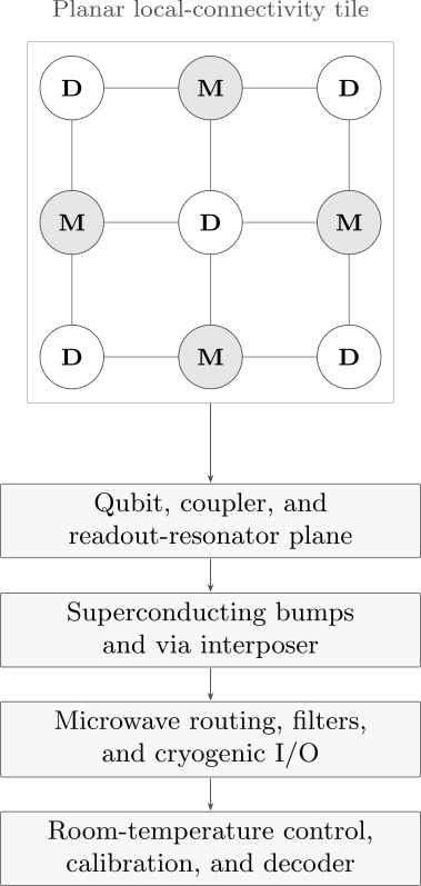
An illustrative architecture, not a unique device blueprint. A planar local-connectivity tile supports repeated parity-check schedules, while dense access to interior qubits motivates vertical interconnects and separate routing layers. The room-temperature controller, calibration service, and decoder are part of the operating system even though they are outside the quantum chip.

Frequency allocation is a graph problem

Transition frequencies cannot be assigned independently. A usable allocation should avoid or control:

• equal or nearly equal neighboring transitions when selectivity requires separation;
• collisions between a qubit’s $0\leftrightarrow1$ transition and a neighbor’s $1\leftrightarrow2$ transition;
• resonances involving couplers, buses, readout modes, sidebands, and multiphoton processes;
• crowded readout resonators on a shared feedline;
• trajectories through unwanted avoided crossings during flux pulses;
• frequencies with strong loss from a defect or package mode.

Fabrication variation turns this into a yield problem. Frequency tunability can recover some devices, but it also changes coherence, residual coupling, readout detuning, and the location of every pulse-dependent collision. Laser trimming, post-fabrication tuning, replaceable modules, and calibration-aware compilation address different parts of the problem.

Parallelism is measured, not inferred

Disjoint graph edges are not automatically executable in parallel. Simultaneous microwave tones can cause Stark shifts, amplifier compression, classical leakage, or spurious transitions. Flux pulses can share return paths or distort neighboring biases. Readout can populate common modes and dephase spectators.

Parallel schedules should be characterized directly. A useful report compares isolated and simultaneous gates, includes spectator states, and records which combinations the compiler forbids. “Nearest-neighbor connectivity” does not specify this concurrency graph.

Packaging, Wiring, and Cryogenics

The qubit mode extends into pads, ground planes, wirebonds, bumps, enclosures, and nearby dielectrics. Packaging is therefore part of the Hamiltonian and loss budget. It must:

• suppress slotline, box, substrate, and interposer modes;
• provide dense ground connections and controlled impedances;
• thermalize conductors while limiting heat flow to the cold stage;
• attenuate incoming thermal noise and infrared radiation;
• route outgoing signals through isolation and low-noise amplification;
• avoid magnetic vortices, dissipative seams, and lossy surface participation;
• remain manufacturable and testable at acceptable yield.

Edge wiring becomes difficult for a large two-dimensional array because interior sites need drive, flux, coupler, and readout access. Air bridges, multilayer wiring, flip-chip bonding, superconducting bumps, through-silicon vias, interposers, and chiplets move signals into the third dimension. Each added layer can also introduce dielectric loss, unwanted modes, thermal resistance, bond variability, and new failure sites.

The refrigerator is a resource ledger. Every cable contributes conducted heat; attenuators dissipate control power; amplifiers and circulators occupy cold volume; readout bandwidth and output power are finite. Cryogenic classical electronics may reduce cable count and latency, but its power, noise, fabrication, and thermal interfaces must be included.

Modularity can reduce die-size and yield pressure. A modular architecture then needs a specified interconnect channel, entanglement rate and fidelity, loss budget, transduction if carriers change, calibration procedure, and routing protocol. Interconnects and Transduction owns that end-to-end channel contract. A successfully bonded chip is not yet a fault-tolerant module.

Modular Architectures owns the next layer: multi-die capability contracts, link inventory, scheduling, distributed error correction, common fault domains, replacement, and sustained service.

Surface-Code Relevance

The Surface Code uses local parity checks on a two-dimensional graph, repeated measurement, reset, and classical decoding. Those requirements align with several strengths of superconducting circuits:

• patterned local couplings;
• fast programmable gates relative to many atomic platforms;
• integrated resonator readout;
• mid-circuit measurement and active reset;
• electronic feedforward and frame tracking;
• planar fabrication compatible with repeated unit cells.

The alignment is not automatic. A useful syndrome cycle also requires:

• a gate order that limits hook errors and crosstalk;
• measurement qubits that reset without contaminating data qubits;
• leakage removal or leakage-aware decoding;
• stable operation over many repeated rounds;
• a decoder whose throughput and tail latency meet the cycle contract;
• correlated-noise characterization;
• logical scaling measured across code distances.

For a rotated planar patch of distance $d$, a common idealized layout uses approximately

$$N_{\mathrm{phys}} = 2d^2-1$$

data and measurement qubits for one logical memory, before routing, boundaries between logical patches, magic-state factories, spares, and other architecture overheads. The formula is a layout count, not a resource estimate for an algorithm.

Dated evidence status

Superconducting processors have progressed from repeated parity checks to surface-code memories in which measured logical error per cycle improves as code distance increases under a stated schedule and decoder. A 2025 experiment reported below-threshold suppression from distance five to distance seven and operated a real-time decoder for the tested logical-memory task.

That result is important evidence for one error-correction stack. It does not by itself demonstrate a universal fault-tolerant computer, algorithm-scale logical error, scalable interconnect yield, magic-state production, or a complete resource budget. The exact device, cycle, decoder, leakage treatment, confidence interval, and acquisition date remain part of the claim. Surface-Code Thresholds explains why “below threshold” is conditional on a code, circuit, noise model, decoder, and scaling family.

Surface codes are not the only route. Subsystem codes, color codes, dynamic circuits, bosonic inner codes, and higher-rate quantum codes trade connectivity, measurement weight, decoder complexity, bias exploitation, and qubit overhead differently. Hardware and code should be co-designed rather than choosing either in isolation.

Scaling the Platform

Scaling changes the optimization target from a best component to a sustained system. The relevant questions include:

1. Fabrication yield: what fraction of junctions, resonators, couplers, bumps, and vias fall inside usable windows?
2. Spectral yield: how many fabricated devices avoid fatal collisions after tuning and trimming?
3. Control fan-out: how many independent waveform, flux, readout, and trigger resources are required?
4. Calibration throughput: can parameters be estimated and validated faster than they drift?
5. Concurrency: what fraction of gates and measurements can run without unacceptable context error?
6. Thermal budget: can attenuation, filtering, amplification, and cryogenic logic operate continuously?
7. Availability: how often is the declared processor subset valid, and how are failed components routed around?
8. Logical evidence: does increasing code size suppress logical error at a useful cycle rate?

Suppose a chip contains $N$ qubits and each requires a serial calibration time $\tau$. The naive time $N\tau$ quickly becomes unacceptable. Local calibration, graph coloring, hierarchical models, shared parameter estimation, drift tracking, and concurrent characterization can reduce wall-clock time, but only if their independence assumptions are tested.

Readout also creates a bandwidth constraint. If $N_m$ measurement channels each produce $b$ raw bits per shot at repetition rate $f_{\mathrm{rep}}$, the uncompressed data rate is

$$R_{\mathrm{raw}} = N_m b f_{\mathrm{rep}}.$$

Early filtering and decoding can reduce exported data, but the cold-to-warm link, digitizers, memory, and processors must still sustain their local streams with bounded latency.

Advantages and Bottlenecks

Architectural advantages

• Electrical design freedom: capacitance, inductance, junction energy, coupling, and port impedance are engineered rather than fixed by an atomic species.
• Fast control cycles: microwave and flux operations can support short gate and feedback schedules when compared under a declared protocol.
• Lithographic integration: qubits, resonators, couplers, filters, and wiring can be patterned and repeated on chip.
• Strong measurement interface: dispersive resonators and parametric amplifiers support single-shot and mid-circuit measurement.
• Programmable interactions: fixed, driven, and tunable couplings support several native-gate families.
• Code–hardware locality match: planar graphs fit repeated low-weight checks without long-range motion.

Persistent bottlenecks

• Materials and interfaces: microscopic loss and fluctuators remain difficult to predict from fabrication data alone.
• Finite anharmonicity and extra modes: fast gates compete with leakage and collision avoidance.
• Frequency crowding and variability: every added component expands the spectral constraint graph.
• Control and readout crosstalk: dense electronics and shared lines create context-dependent errors.
• Cryogenic fan-out: cables, attenuators, filters, amplifiers, and heat load scale with the control architecture.
• Packaging and yield: three-dimensional integration must preserve coherence while adding many bonds and vias.
• Correlated rare events: radiation, quasiparticles, heating, or common electronics can violate independent-error models.
• Calibration burden: a large processor is a drifting coupled system, not a static table of independently tuned qubits.

These are engineering and physics constraints, not arguments that progress is impossible. Conversely, isolated record values do not show that the constraints have been solved simultaneously.

Worked Architecture Audit

Consider a transmon design with

$$\frac{E_C}{h} = 250\,\mathrm{MHz}, \qquad \frac{E_J}{E_C} = 50.$$

Then $E_J/h=12.5\,\mathrm{GHz}$, and the leading transmon estimate gives

$$\begin{aligned} \frac{\omega_{01}}{2\pi} &\approx \frac{\sqrt{8E_JE_C}-E_C}{h} \\ &= 5.00\,\mathrm{GHz} - 0.25\,\mathrm{GHz} \\ &= 4.75\,\mathrm{GHz}, \end{aligned}$$

with

$$\frac{\alpha}{2\pi} \approx -250\,\mathrm{MHz}.$$

This is a design estimate. Spectroscopy must identify the actual transitions, nearby modes, and device-to-device spread.

At equilibrium temperature $T=20\,\mathrm{mK}$, the ideal two-level population ratio is

$$\frac{p_1}{p_0} = \exp\!\left( -\frac{h(4.75\,\mathrm{GHz})} {k_{\mathrm B}(20\,\mathrm{mK})} \right) \approx 1.1\times10^{-5}.$$

At an effective temperature of $60\,\mathrm{mK}$, the same ratio is about $2.2\times10^{-2}$. This large difference is why base temperature cannot substitute for qubit thermometry. Even an effective-temperature fit is only a model when quasiparticle or drive-induced populations are present.

Now suppose $T_1=150\,\mu\mathrm{s}$ and a repeated syndrome cycle lasts $t_c=1.1\,\mu\mathrm{s}$. A qubit held in $\lvert1\rangle$ for the full cycle would relax with probability

$$\begin{aligned} p_{\mathrm{relax}} &= 1-e^{-t_c/T_1} \\ &\approx 7.3\times10^{-3}. \end{aligned}$$

If its average excited-state occupancy during the schedule were $q=0.4$, the rough occupancy-weighted contribution would be

$$q\,p_{\mathrm{relax}} \approx 2.9\times10^{-3}.$$

This is neither a complete gate error nor a logical error. It omits dephasing, control faults, measurement, reset, leakage, crosstalk, correlations, and the exact time-dependent state. The calculation nevertheless reveals a systems constraint: gate speed, cycle schedule, and coherence must be compared on the same timeline.

Evidence and Reporting Ledger

A mature superconducting-hardware report should provide:

Claim layer	Minimum evidence
qubit mode	spectroscopy, anharmonicity, matrix-element or model checks, unwanted-mode search
initialization	unconditional populations, reset duration, leakage and spectator effects
one-qubit gate	pulse definition, calibration, leakage, held-out and simultaneous benchmarking
two-qubit gate	coupling context, residual interactions, spectators, leakage, full compiled duration
readout	assignment matrix, QND or state-preservation test, latency, reset, multiplexed context
processor	active yield, connectivity, concurrency map, drift and availability
error correction	repeated schedule, decoder, detection statistics, logical error with uncertainty, distance scaling

Report dates and distributions, not only a best device. Separate a component demonstrated once from a process reproduced across wafers, cooldowns, modules, and operating days. For active or proprietary systems, missing calibration, postselection, and disabled-component information should limit the conclusion rather than be silently guessed.

Common Mistakes

• Calling every superconducting qubit a transmon. Flux qubits, fluxonium, protected circuits, and bosonic modes have different Hamiltonians and control contracts.
• Treating the qubit as exactly two level. Leakage and multilevel dispersive physics are central architecture constraints.
• Equating refrigerator temperature with qubit temperature. The electromagnetic and quasiparticle environments may be out of equilibrium.
• Assuming a sweet spot removes noise. It removes selected first-order sensitivity, not all dephasing or relaxation.
• Comparing gate time directly with one coherence number. Driven, idle, simultaneous, and measured schedules sample different noise and occupancy.
• Using average gate fidelity as an error probability. Coherent error, leakage, correlation, and context can compose differently.
• Treating a tunable coupler as a classical switch. It is an additional quantum mode with calibration and leakage paths.
• Calling assignment fidelity QND fidelity. Correct labels do not establish conditional state preservation.
• Counting designed edges as usable parallel connectivity. Residual interactions and scheduling exclusions change the graph.
• Treating lithography as automatic scalability. yield, packaging, cold I/O, calibration, and correlated noise remain system constraints.
• Calling one below-threshold memory a complete fault-tolerant computer. Universal logical operations and full resource scaling require additional evidence.
• Comparing vendor headline numbers without a common metric contract. Device, protocol, date, uncertainty, and workload must match.

Exercises

1. Estimate a transmon spectrum

A transmon has $E_C/h=220\,\mathrm{MHz}$ and $E_J/E_C=60$. Estimate $\omega_{01}/2\pi$ and $\alpha/2\pi$ using the leading large-$E_J/E_C$ formulas.

Solution

First,

$$\frac{E_J}{h} = 60(0.220\,\mathrm{GHz}) = 13.2\,\mathrm{GHz}.$$

Therefore

$$\begin{aligned} \frac{\omega_{01}}{2\pi} &\approx \sqrt{8(13.2)(0.220)}\,\mathrm{GHz} \\ &\quad - 0.220\,\mathrm{GHz} \\ &\approx 4.60\,\mathrm{GHz}. \end{aligned}$$

The anharmonicity estimate is

$$\frac{\alpha}{2\pi} \approx -\frac{E_C}{h} = -220\,\mathrm{MHz}.$$

These are asymptotic design values. A circuit model and spectroscopy are needed for precision and for identifying other modes.

2. Compare equilibrium populations

For a $5.0\,\mathrm{GHz}$ two-level transition, estimate the equilibrium excited-state population at $20\,\mathrm{mK}$ and $60\,\mathrm{mK}$.

Solution

For a two-level system,

$$p_1 = \frac{1} {1+e^{hf/(k_{\mathrm B}T)}}.$$

Since $hf/k_{\mathrm B}\approx0.240\,\mathrm K$, at $20\,\mathrm{mK}$,

$$p_1 \approx \frac{1}{1+e^{12.0}} \approx 6.1\times10^{-6}.$$

At $60\,\mathrm{mK}$,

$$p_1 \approx \frac{1}{1+e^{4.00}} \approx 1.8\times10^{-2}.$$

The threefold temperature increase changes the equilibrium population by roughly three orders of magnitude. A measured population need not be thermal, so this comparison is a diagnostic model rather than proof of a temperature.

3. Verify a flux sweet spot

For the effective flux-qubit splitting

$$E(\delta\Phi) = \sqrt{ \Delta^2 + (2I_p\delta\Phi)^2 },$$

show that $\delta\Phi=0$ is first-order insensitive to flux and find the leading small-$\delta\Phi$ correction.

Solution

Differentiation gives

$$\frac{dE}{d(\delta\Phi)} = \frac{4I_p^2\delta\Phi} {\sqrt{\Delta^2+(2I_p\delta\Phi)^2}},$$

which vanishes at $\delta\Phi=0$. Expanding the square root,

$$\begin{aligned} E(\delta\Phi) &= \Delta \sqrt{ 1+ \frac{4I_p^2\delta\Phi^2}{\Delta^2} } \\ &\approx \Delta + \frac{2I_p^2}{\Delta} \delta\Phi^2. \end{aligned}$$

The linear sensitivity is removed, but quadratic flux sensitivity and other noise channels remain.

4. Accumulate residual conditional phase

Two idle qubits have residual interaction

$$\frac{H_{ZZ}}{\hbar} = \frac{\zeta}{4}Z_1Z_2, \qquad \frac{\zeta}{2\pi} = 50\,\mathrm{kHz}.$$

What conditional phase magnitude accumulates during $2.0\,\mu\mathrm{s}$?

Solution

For this convention, the two-qubit conditional phase magnitude is $\lvert\zeta t\rvert$. Thus

$$\begin{aligned} \lvert\phi_{ZZ}\rvert &= 2\pi (50\times10^3) (2.0\times10^{-6}) \\ &= 0.2\pi \approx 0.628\,\mathrm{rad}. \end{aligned}$$

That is not negligible. An echo, calibrated frame or phase compensation, coupler bias, or schedule change must account for it. Spectator-state dependence should also be tested.

5. Estimate a simple Purcell limit

In the ideal two-level dispersive estimate,

$$\Gamma_{\mathrm P} \approx \kappa \left( \frac{g}{\Delta} \right)^2.$$

Take $g/2\pi=100\,\mathrm{MHz}$, $\lvert\Delta\rvert/2\pi=1.0\,\mathrm{GHz}$, and $\kappa/2\pi=5.0\,\mathrm{MHz}$. Estimate the Purcell-limited $T_1$.

Solution

The mixing ratio is $g/\lvert\Delta\rvert=0.1$, so

$$\frac{\Gamma_{\mathrm P}}{2\pi} \approx (5.0\,\mathrm{MHz})(0.1)^2 = 50\,\mathrm{kHz}.$$

Consequently,

$$T_{1,\mathrm P} = \frac{1}{\Gamma_{\mathrm P}} \approx \frac{1}{2\pi(50\,\mathrm{kHz})} \approx 3.2\,\mu\mathrm{s}.$$

This deliberately simple result shows the readout-speed tradeoff. Multilevel corrections and the actual frequency-dependent impedance, including a Purcell filter, are required for device design.

6. Bound relaxation during a cycle

A qubit has $T_1=200\,\mu\mathrm{s}$, a syndrome cycle lasts $1.0\,\mu\mathrm{s}$, and its average excited-state occupancy during the schedule is $q=0.5$. Estimate the occupancy-weighted relaxation contribution.

Solution

For full excited-state occupancy,

$$\begin{aligned} p_{\mathrm{relax}} &= 1-e^{-1/200} \\ &\approx 4.99\times10^{-3}. \end{aligned}$$

Weighting by $q$ gives

$$q\,p_{\mathrm{relax}} \approx 2.49\times10^{-3}.$$

This is a schedule-level estimate, not a logical error probability. The exact state history, gate errors, dephasing, measurement, leakage, and decoder response still matter.

7. Color a square coupling graph

Show why two alternating qubit-frequency bands can separate every nearest-neighbor pair on an ideal square lattice. Then name two reasons that this does not solve frequency allocation for a transmon processor.

Solution

The square lattice is bipartite: color each vertex by the parity of its integer coordinates. Every nearest-neighbor edge joins opposite parity, so assigning frequency band $A$ to one color and $B$ to the other makes neighboring $0\leftrightarrow1$ bands different.

This does not control collisions involving $1\leftrightarrow2$ transitions, couplers, readout resonators, sidebands, or multiphoton processes. It also leaves same-band next-nearest neighbors that can interact through crosstalk or shared modes. Fabrication spread broadens both bands, and simultaneous-gate protocols may require more than pairwise separation.

8. Budget multiplexed readout bandwidth

An amplifier offers $600\,\mathrm{MHz}$ of usable bandwidth. Each readout channel, including its guard band, is allocated $30\,\mathrm{MHz}$. What is the naive maximum channel count, and why is it only an upper bound?

Solution

The arithmetic allocation is

$$N_{\max} = \left\lfloor \frac{600}{30} \right\rfloor = 20.$$

Actual yield can be lower because resonator frequencies vary, linewidths and ring-down times differ, amplifier gain and phase are not flat, total power can compress the chain, intermodulation products appear, and qubit-state-dependent shifts or neighboring resonators can collide. Classifier correlation and Purcell-filter response must also be validated.

9. Separate assignment from state preservation

A readout reports the prepared computational-basis label correctly $99.5\%$ of the time. Repeating the measurement gives the same label $99.7\%$ of the time. Does this establish $99.7\%$ quantum non-demolition fidelity?

Solution

No. Repeated-label agreement combines detector assignment, state change during and between measurements, relaxation, excitation, leakage, and detector memory. A biased or correlated classifier can repeat the same wrong label.

A stronger test estimates the conditional postmeasurement state using independently calibrated subsequent measurements, varies the delay, separates upward and downward transitions, includes leakage outcomes, and models detector correlations. The POVM and conditional instrument are different objects.

10. Audit a below-threshold claim

A report states that a larger surface-code memory had lower logical error per cycle than a smaller one on a superconducting processor. List what must be checked before concluding that scalable fault-tolerant computation has been demonstrated.

Solution

Check the code distances and layouts, number of rounds, prepared logical states, complete syndrome circuit, active qubit subset, decoder and whether it ran online, leakage and reset treatment, postselection, uncertainty, drift, and whether the comparison used matched conditions. Verify that logical suppression persists over repeated cycles and is not a finite-sample or selected-subset effect.

Even valid below-threshold memory scaling does not establish universal fault-tolerant logical gates, state injection and magic-state production, algorithm-level logical error, module and wiring yield, sustained availability, or a complete physical-resource estimate. The demonstrated claim should remain a logical-memory result under its stated operating contract.

References

1. Y. Nakamura, Y. A. Pashkin, and J. S. Tsai, “Coherent control of macroscopic quantum states in a single-Cooper-pair box,” Nature 398, 786–788 (1999), doi:10.1038/19718.
2. J. E. Mooij, T. P. Orlando, L. Levitov, L. Tian, C. H. van der Wal, and S. Lloyd, “Josephson persistent-current qubit,” Science 285, 1036–1039 (1999), doi:10.1126/science.285.5430.1036.
3. J. Koch et al., “Charge-insensitive qubit design derived from the Cooper pair box,” Physical Review A 76, 042319 (2007), doi:10.1103/PhysRevA.76.042319.
4. V. E. Manucharyan, J. Koch, L. I. Glazman, and M. H. Devoret, “Fluxonium: Single Cooper-pair circuit free of charge offsets,” Science 326, 113–116 (2009), doi:10.1126/science.1175552.
5. A. Blais, R.-S. Huang, A. Wallraff, S. M. Girvin, and R. J. Schoelkopf, “Cavity quantum electrodynamics for superconducting electrical circuits: An architecture for quantum computation,” Physical Review A 69, 062320 (2004), doi:10.1103/PhysRevA.69.062320.
6. M. H. Devoret and R. J. Schoelkopf, “Superconducting circuits for quantum information: An outlook,” Science 339, 1169–1174 (2013), doi:10.1126/science.1231930.
7. P. Krantz et al., “A quantum engineer’s guide to superconducting qubits,” Applied Physics Reviews 6, 021318 (2019), doi:10.1063/1.5089550.
8. M. Kjaergaard et al., “Superconducting qubits: Current state of play,” Annual Review of Condensed Matter Physics 11, 369–395 (2020), doi:10.1146/annurev-conmatphys-031119-050605.
9. A. Blais, A. L. Grimsmo, S. M. Girvin, and A. Wallraff, “Circuit quantum electrodynamics,” Reviews of Modern Physics 93, 025005 (2021), doi:10.1103/RevModPhys.93.025005.
10. A. Gyenis et al., “Moving beyond the transmon: Noise-protected superconducting quantum circuits,” PRX Quantum 2, 030101 (2021), doi:10.1103/PRXQuantum.2.030101.
11. R. A. Mencia, W.-J. Lin, H. Cho, M. G. Vavilov, and V. E. Manucharyan, “Integer fluxonium qubit,” PRX Quantum 5, 040318 (2024), doi:10.1103/PRXQuantum.5.040318.
12. J. M. Chow et al., “Simple all-microwave entangling gate for fixed-frequency superconducting qubits,” Physical Review Letters 107, 080502 (2011), doi:10.1103/PhysRevLett.107.080502.
13. D. C. McKay et al., “Universal gate for fixed-frequency qubits via a tunable bus,” Physical Review Applied 6, 064007 (2016), doi:10.1103/PhysRevApplied.6.064007.
14. F. Yan et al., “Tunable coupling scheme for implementing high-fidelity two-qubit gates,” Physical Review Applied 10, 054062 (2018), doi:10.1103/PhysRevApplied.10.054062.
15. J. Gambetta, W. A. Braff, A. Wallraff, S. M. Girvin, and R. J. Schoelkopf, “Protocols for optimal readout of qubits using a continuous quantum nondemolition measurement,” Physical Review A 76, 012325 (2007), doi:10.1103/PhysRevA.76.012325.
16. T. Walter et al., “Rapid high-fidelity single-shot dispersive readout of superconducting qubits,” Physical Review Applied 7, 054020 (2017), doi:10.1103/PhysRevApplied.7.054020.
17. J. M. Martinis et al., “Decoherence in Josephson qubits from dielectric loss,” Physical Review Letters 95, 210503 (2005), doi:10.1103/PhysRevLett.95.210503.
18. G. Catelani, R. J. Schoelkopf, M. H. Devoret, and L. I. Glazman, “Relaxation and frequency shifts induced by quasiparticles in superconducting qubits,” Physical Review B 84, 064517 (2011), doi:10.1103/PhysRevB.84.064517.
19. A. P. M. Place et al., “New material platform for superconducting transmon qubits with coherence times exceeding $0.3$ milliseconds,” Nature Communications 12, 1779 (2021), doi:10.1038/s41467-021-22030-5.
20. D. R. W. Yost et al., “Solid-state qubits integrated with superconducting through-silicon vias,” npj Quantum Information 6, 59 (2020), doi:10.1038/s41534-020-00289-8.
21. D. Rosenberg et al., “3D integrated superconducting qubits,” npj Quantum Information 3, 42 (2017), doi:10.1038/s41534-017-0044-0.
22. J. Kelly et al., “State preservation by repetitive error detection in a superconducting quantum circuit,” Nature 519, 66–69 (2015), doi:10.1038/nature14270.
23. Google Quantum AI and Collaborators, “Quantum error correction below the surface code threshold,” Nature 638, 920–926 (2025), doi:10.1038/s41586-024-08449-y.

Further Connections

• Hardware Overview compares this platform with trapped ions, neutral atoms, photons, spins, bosonic modes, and topological proposals under one contract.
• Metrics for Quantum Hardware defines coherence, gate, leakage, readout, crosstalk, logical, and workload metrics without collapsing them into one score.
• Control, Readout, and Calibration develops waveform delivery, detector inference, dependency-aware calibration, drift monitoring, and feedback.
• Pulse-Level Control develops the frame, DRAG, sampling, scheduling, transfer, and qualification contracts used to compile microwave and flux controls.
• Interconnects and Transduction develops direct microwave links, optical conversion, heralded services, added-noise accounting, and modular evidence.
• Modular Architectures develops multi-die service contracts, deterministic and heralded fabrics, pair inventory, routing, fault domains, and modular logical evidence.
• Cryogenic and Vacuum Infrastructure develops the refrigerator-stage, wiring, attenuation, shielding, radiation, diagnostics, and uptime contract beneath a superconducting processor.
• Materials and Fabrication Interface connects dielectric participation, junction dispersion, wafer-scale process variation, predictive screening, graph-aware yield, aging, and calibration burden to processor evidence.
• Circuit QED Overview owns the detailed transmon, resonator, dispersive-readout, Purcell, and cryogenic-chain derivations.
• Josephson Effect supplies the junction and SQUID physics beneath the circuit models.
• One-Over-F Noise explains low-frequency noise, protocol-dependent dephasing, and filter-function interpretation.
• Quantum Instruments separates detector outcomes from conditional state updates and repeated-measurement behavior.
• Surface Code owns planar patches, repeated syndrome extraction, decoding, thresholds, lattice surgery, and resource overhead.
• Surface-Code Thresholds states the assumptions required to infer logical suppression from physical error models and finite-size experiments.