Quantum Memories

A quantum memory accepts a quantum state, preserves its operationally relevant information for a declared interval, and returns that information on a useful carrier. Ideally, the write–store–read process implements the identity channel, possibly followed by a known change of basis, frequency, or physical encoding.

Long coherence is necessary for many memories, but it is not sufficient. A nuclear spin can remain coherent for hours while coupling too weakly or slowly to accept an incoming photonic qubit. An optical delay can release a pulse with high fidelity while offering no genuinely on-demand readout. A memory can return the surviving states with excellent conditional fidelity while losing most inputs. A large multimode count can use fixed-time echoes that do not satisfy a repeater scheduler.

The complete device is therefore a channel with an interface, not merely a quiet degree of freedom. Trustworthy comparison keeps efficiency, fidelity, storage time, bandwidth, mode capacity, noise, latency, and duty cycle visible at the same time.

Purpose and Canonical Scope

This page owns the hardware-neutral architecture of quantum memories:

• the write, storage, control, and read maps;
• optical ensemble, single-emitter, spin, oscillator, acoustic, and photonic buffer technologies;
• electromagnetically induced transparency, Raman, gradient-echo, controlled rephasing, atomic-frequency-comb, cavity, swap, and active-correction mechanisms;
• efficiency, conditional and unconditional fidelity, lifetime, bandwidth, time–bandwidth product, noise, multimode capacity, and on-demand control;
• dephasing, loss, control-pulse noise, spectral diffusion, mode mismatch, cross-talk, and decoder faults;
• evidence labels through 10 August 2026.

Quantum Channels and Noise owns completely positive maps, Kraus representations, and channel composition. Erasure and Loss Channels and Dephasing Channel own the canonical channel derivations. Electromagnetically Induced Transparency and Cavity QED own the detailed light–matter physics. This article asks how those mechanisms become a usable memory service.

Quantum Repeaters owns queueing, synchronization, repeater scheduling, and service-level requirements; it links here rather than duplicating the hardware protocols. Quantum Network Architectures uses memory slots as leased, identified network resources and owns their multiuser reservation, routing, and administrative semantics. Quantum Teleportation already owns the canonical protocol for transferring an unknown state using entanglement and classical communication.

The Memory Channel

Write the end-to-end memory map at storage time $t$ as

$$\mathcal M_t = \mathcal R \circ \mathcal S_t \circ \mathcal W.$$

Here $\mathcal W$ writes the input carrier into the storage degree of freedom, $\mathcal S_t$ describes storage plus applied control, and $\mathcal R$ returns an output carrier. The ideal target may include a known unitary $U_t$, frequency conversion, or a change from a photonic to a stationary encoding and back.

A simple flagged-erasure model is

$$\mathcal M_t(\rho) = \eta(t) U_t\rho U_t^\dagger + \left[ 1-\eta(t) \right] \lvert e\rangle\langle e\rvert,$$

where $\lvert e\rangle$ is orthogonal to the computational output space. This model cleanly separates efficiency $\eta$ from the state quality on successful retrieval. Real memories add dephasing, state-dependent loss, background photons, leakage, mode distortion, and imperfect erasure flags.

A memory is more than a delay

A passive delay line implements a predetermined release time. A fully on-demand memory permits a controller to choose the read time after the write event, within a stated acceptance window. Intermediate devices include:

• fixed-delay fibre, cavity, or echo buffers;
• switchable loops with release only at discrete circulation times;
• memories with a fixed rephasing delay plus a programmable spin-wave dwell;
• random-access banks with independently addressable cells;
• stationary qubits that remain in place while the processor schedules later gates.

Each can be useful. The name should state which timing service is actually available.

The Architecture Contract

Represent a memory module as

$$\mathcal A_{\rm mem} = \left( \mathcal I, \mathcal W, \mathcal H_{\rm s}, \mathcal C, \mathcal R, \mathcal V \right).$$

Here $\mathcal I$ is the input mode and impedance-matching layer, $\mathcal H_{\rm s}$ the storage subsystem, $\mathcal C$ the protection and timing controller, and $\mathcal V$ the verification, heralding, or erasure flag. A complete description identifies:

1. the input ensemble and physical mode functions;
2. the write and read mechanisms and their reference planes;
3. the storage basis and all spectator levels or modes;
4. fixed-delay, gated, or fully on-demand timing behavior;
5. write, storage, and read efficiencies separately;
6. conditional fidelity and unconditional channel behavior;
7. storage lifetime under the actual control sequence;
8. accepted bandwidth, pulse duration, and spectral compatibility;
9. temporal, spectral, spatial, and polarization mode capacity;
10. background noise, false heralds, cross-talk, duty cycle, and reset;
11. classical latency and scheduling constraints;
12. every converter, filter, cavity, switch, cryostat, laser, microwave line, detector, control pulse, and rejected trial inside the resource boundary.

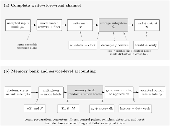
A memory claim begins at the accepted input mode and ends at the usable output, not at an internal coherence measurement. The write, protected storage, read, filtering, heralding, scheduler, and verification layers all contribute to $\eta(t)$, channel fidelity, noise, latency, and accepted throughput.

Performance Vector

No scalar ranks quantum memories for every task. A useful performance record is

$$\mathbf m = \left( \eta, F, T_{\rm s}, B, M, p_{\rm n}, \tau_{\rm wr}, D \right),$$

where $\eta$ is end-to-end efficiency, $F$ an ensemble-appropriate fidelity, $T_{\rm s}$ storage time, $B$ accepted bandwidth, $M$ independently useful mode capacity, $p_{\rm n}$ noise probability, $\tau_{\rm wr}$ write/read latency, and $D$ duty factor. Correlations and trade-offs among these entries matter more than isolated records.

Efficiency

For an optical memory, a common end-to-end definition is

$$\eta(t) = \frac{N_{\rm retrieved}(t)} {N_{\rm accepted\ input}},$$

with both counts referred to declared spatial, spectral, temporal, and polarization modes. The report should distinguish:

$$\eta = \eta_{\rm in} \eta_{\rm write} \eta_{\rm store}(t) \eta_{\rm read} \eta_{\rm out},$$

where the product notation means that each factor is a conditional efficiency. Correcting away coupling, filtering, or detector loss can help diagnose a component but does not describe the state available to the next network or processor module.

Fidelity

Conditional fidelity asks how well the retrieved state matches the target, given a declared success event:

$$F_{\rm cond} = \int d\psi\, \langle\psi| U_t^\dagger \rho_{\rm out}^{(\psi)} U_t |\psi\rangle.$$

The integral and prior define the input ensemble. Uniform qubits, coherent states with a Gaussian prior, squeezed states, and a finite alphabet have different classical measure-and-prepare benchmarks.

For a trace-preserving qubit channel, entanglement fidelity can be measured by storing half of a maximally entangled state:

$$F_{\rm e} = \langle\Phi| \left( \mathcal I\otimes U_t^\dagger\circ\mathcal M_t \right) \left( \lvert\Phi\rangle\langle\Phi\rvert \right) |\Phi\rangle.$$

The average pure-state fidelity then obeys

$$F_{\rm avg} = \frac{2F_{\rm e}+1}{3}.$$

Postselection and erasure require care: a high fidelity on rare retrieved events does not imply a high-fidelity trace-preserving channel.

Quantum benchmarks

For a uniformly distributed unknown pure qubit, an optimal measure-and-prepare memory has average fidelity at most $2/3$. That number is not universal. The benchmark changes with the prior, input energy, accepted loss, and whether unsuccessful outcomes are allowed.

A valid quantum-memory claim therefore states:

• the tested input ensemble and its prior;
• whether the benchmark includes the measured efficiency;
• whether vacuum and no-click events enter the score;
• whether fidelity is raw, background-subtracted, or loss-corrected;
• confidence intervals and any optimized classical strategy.

Storage time and lifetime

$T_1$, Ramsey $T_2^*$, echo $T_2$, and dynamically decoupled coherence time describe different experiments. The useful memory lifetime is the interval over which the complete write–read channel meets a task threshold.

For a qubit undergoing pure dephasing with coherence factor $\lambda(t)=e^{-t/T_2}$,

$$F_{\rm avg}(t) = \frac{2+\lambda(t)}{3}.$$

Population loss, control-pulse errors, state-dependent retrieval, and background counts can make the measured memory decay differ from this simple curve.

Bandwidth and time–bandwidth product

The accepted bandwidth $B$ and storage time define

$$\mathcal B = B T_{\rm s}.$$

This time–bandwidth product is an upper-scale indicator for temporal mode capacity, not an automatic count of independently stored qubits. Actual mode capacity also depends on pulse shape, guard intervals, control bandwidth, cross-talk, retrieval ordering, and signal-to-noise ratio.

Noise and the single-photon regime

For a memory with unconditional output-noise probability $p_{\rm n}$ per accepted mode, a useful scale is

$$\mu_1 = \frac{p_{\rm n}}{\eta},$$

the mean input photon number that would give signal-to-noise ratio near one in a simple linear model. Noise must be measured with the same preparation, control, filtering, retrieval window, and detector gates used for storage.

Collective Optical Memories

Atomic ensembles enhance light–matter coupling by storing one optical excitation as a collective spin wave. A schematic single-excitation state is

$$\lvert1_{\rm s}\rangle = \frac{1}{\sqrt N} \sum_{j=1}^{N} e^{i\Delta\mathbf k\cdot\mathbf r_j} \lvert g_1\cdots s_j\cdots g_N \rangle.$$

The phase pattern $\Delta\mathbf k$ records the input and control wavevectors. Directional retrieval follows from collective interference. Atomic motion, field gradients, collisions, and spatially varying light shifts dephase this pattern.

Electromagnetically induced transparency

In a three-level lambda system, a control field opens a transparency window for the signal and converts the propagating field into a dark-state polariton. Schematically,

$$\Psi_{\rm D} = \cos\theta\,\mathcal E - \sin\theta\,S,$$

where $\mathcal E$ is the optical mode and $S$ a collective spin coherence. Adiabatically reducing the control field rotates the polariton into matter; restoring the control retrieves it.

EIT memories can provide on-demand readout and excellent state fidelity. Their efficiency depends on optical depth, control shaping, decoherence, and mode matching. The transparency bandwidth can be narrow, and strong control fields can add leakage, fluorescence, and four-wave-mixing noise.

Off-resonant Raman storage

Raman memories detune the optical fields from the excited state and transfer the signal to a spin wave through a two-photon process. Large detuning can support broader bandwidth and reduce resonant absorption, but stronger control energy may be required. Spontaneous Raman scattering and four-wave mixing can dominate single-photon-level noise.

EIT and Raman operation are limiting regimes of a broader light–matter interface. The meaningful choice depends on bandwidth, optical depth, detuning, control power, and noise, rather than protocol name alone.

Gradient echo and controlled broadening

Controlled reversible inhomogeneous broadening maps different frequency components to different atomic detunings. Reversing the detuning gradient reverses dephasing and produces an echo. Gradient echo memory can offer high efficiency and pulse sequencing, especially in warm vapours and inhomogeneously broadened solids.

The reversal operation must preserve phase and avoid population inversion that would amplify spontaneous noise. A classical echo is not automatically a quantum memory; the retrieved field must beat the relevant classical benchmark and preserve nonclassical correlations.

Atomic-frequency-comb storage

An atomic-frequency-comb memory prepares a periodic absorption profile with tooth spacing $\Delta$ in hertz. Absorbed frequency classes dephase and then rephase at

$$t_{\rm echo} = \frac{1}{\Delta}.$$

The basic AFC echo is a fixed-delay memory. Applying a control pulse before the echo transfers optical coherence to a long-lived spin state; a later control pulse restores it and provides on-demand spin-wave storage.

AFC memories are naturally temporally multimode because many pulses can be absorbed before the common rephasing time. Rare-earth-doped crystals also offer broad inhomogeneous lines for spectral multiplexing. Spin-wave control adds noise and transfer loss, so fixed-delay mode-count records and on-demand single-photon records should not be compared as the same service.

Single Emitters and Small Registers

A single atom, ion, molecule, quantum dot, or colour centre can store a qubit in long-lived internal states. A cavity or nanophotonic resonator enhances the interaction with a selected optical mode. The cooperativity

$$C = \frac{4g^2}{\kappa\gamma}$$

compares coherent coupling $g$ with cavity decay $\kappa$ and emitter decay $\gamma$. Large cooperativity improves reflection, absorption, and spin–photon gate probabilities, but useful performance also needs spectral stability, mode matching, collection, control, and reset.

Single-emitter memories offer:

• individually addressable qubits;
• local gates and nondestructive readout;
• heralded remote entanglement;
• compact registers with communication and storage qubits;
• direct integration with error detection.

Their bottlenecks include photon collection, indistinguishability, narrow bandwidth, spectral diffusion, fabrication variability, and probabilistic remote links.

Communication and storage qubits

A network node often separates a fast optical communication qubit from a long-lived storage qubit. An electron spin can couple strongly to a photon, while a nearby nuclear spin stores entanglement during later attempts. The local transfer and repeated optical excitation must not destroy the stored state.

Defect and Solid-State Spin Qubits owns the detailed SiV, NV, silicon-vacancy, rare-earth, and nuclear-register architectures. This page owns the memory-channel test applied to them.

Trapped atoms and ions

Hyperfine or clock-state qubits in trapped ions and neutral atoms can have very long coherence and high-fidelity control. Optical cavities or high-numerical-aperture collection provide flying-photon interfaces. Trapped-ion experiments have demonstrated hour-scale estimated coherence for a protected single qubit, while remote entanglement experiments test the fuller interface-plus-memory service.

A one-qubit coherence record does not establish a bank with simultaneous write, random access, cross-talk control, photonic interfacing, and repeated network operation.

Solid-State Ensemble Memories

Rare-earth ions in crystals combine narrow homogeneous transitions, large inhomogeneous bandwidth, long hyperfine coherence, and compatibility with photon-echo protocols. The crystal is stationary and naturally supports many spectral and temporal modes. Waveguides, cavities, and fibre doping can improve integration.

The costs are substantial:

• cryogenic operation;
• spectral-hole-burning preparation;
• narrow or material-specific wavelengths;
• magnetic-field stabilization;
• imperfect control-pulse transfer;
• fluorescence and free-induction-decay noise;
• spectral diffusion and instantaneous spectral diffusion;
• frequency conversion for telecom networks.

In 2021, a europium-doped crystal stored coherent optical fields for one hour using spin-wave AFC, a zero-first-order-Zeeman field, and dynamical decoupling. Time-bin-like interference after one hour had reported fidelity near $96\%$. The inputs were bright coherent probe pulses, not arbitrary single-photon qubits. The result established an extraordinary coherent storage-time capability, not an hour-long high-efficiency single-photon network memory.

Microwave, Oscillator, and Acoustic Memories

Superconducting processors often use high-quality microwave cavities as storage modes and nonlinear qubits as controllers. A beam-splitter-like interaction between modes,

$$H_{\rm swap} = \hbar g \left( a^\dagger b+ab^\dagger \right),$$

transfers a state after an ideal interaction time

$$t_{\rm swap} = \frac{\pi}{2g}.$$

Three-dimensional cavities have reached millisecond photon lifetimes, while bosonic encodings and repeated parity checks can extend logical storage beyond the lifetime of constituent error processes. Bosonic Qubits owns those encoded architectures and break-even experiments.

Other proposals and experiments use:

• spin ensembles coupled to microwave resonators;
• acoustic and mechanical modes;
• magnonic modes;
• long superconducting transmission lines;
• microwave-to-optical transducers connected to optical memories.

Strong coupling, state-transfer fidelity, thermal occupation, mode crowding, and transduction loss determine whether a long-lived mode is useful. Interconnects and Transduction owns the converter and complete-link contract; this page owns the write–store–read channel on either side of that interface.

Active and Error-Corrected Memories

A passive memory suppresses noise through isolation, clock transitions, material quality, or a Hamiltonian gap. An active memory repeatedly detects errors and applies recovery or updates a frame.

For a logical memory, the central benchmark is not physical $T_1$ or $T_2$. It is logical survival under repeated correction:

$$\epsilon_L(d,t) = 1-F_L(d,t),$$

measured versus code distance or another resource parameter $d$ at matched storage time and operation conditions. Fault-tolerant evidence requires $\epsilon_L$ to decrease as the code grows, with syndrome extraction, decoding, leakage, reset, and acceptance included.

Dynamical decoupling is not quantum error correction. It averages selected Hamiltonian noise using open-loop pulses; it does not generally identify which error occurred. Conversely, an error-corrected memory can be harmed by noisy syndrome cycles even when its physical storage mode is excellent.

Dynamical Decoupling owns filter functions and sequence design.

Dynamical Decoupling for quantum-information deployment owns compiled memory-window placement, frame-aware action, control cost, and held-out unconditional benefit; this page retains the end-to-end write–store–read memory-service claim.

Metrics for Quantum Hardware owns logical benchmarking principles.

Photonic Loops and Buffers

Switchable fibre or integrated-waveguide loops can store a photonic qubit without converting it to matter. They can be broadband, encoding-agnostic, and simple to interface. If each circulation has transmission $\eta_{\rm c}$, then after $N$ cycles

$$\eta_N = \eta_{\rm in} \eta_{\rm c}^{N} \eta_{\rm out}.$$

The exponential loss makes long storage difficult. Polarization rotation, dispersion, switch leakage, phase noise, and timing jitter accumulate as well. A 2025 fibre-coupled loop-and-switch experiment reported about $54\%$ pass-through efficiency and storage efficiency scaling approximately as $0.5^{N+1}$. This is a useful broadband buffer demonstration and a clear example of why cycle-resolved loss must accompany fidelity.

Multiplexing and Random Access

Memory multiplexing can use:

• temporal modes: many pulses before retrieval;
• spectral modes: independently addressed frequency bins;
• spatial modes: separate cells, wavevectors, or emitters;
• polarization modes: often implemented as two balanced rails;
• orbital or high-dimensional modes: qudits stored in a mode basis;
• hybrid modes: products of several degrees of freedom.

For $M$ independent attempts with success probability $p$, the probability that at least one succeeds is

$$p_{\geq1} = 1-(1-p)^M.$$

The benefit is real only if the successful mode can be identified, preserved, and routed with low cross-talk and acceptable latency. A total mode count must therefore include:

• per-mode efficiency and fidelity distributions;
• cross-talk matrix;
• simultaneous versus sequential addressability;
• fixed versus on-demand retrieval;
• mode-dependent storage time;
• demultiplexer loss;
• controller and detector throughput.

In 2025, a praseodymium-doped crystal array combined ten spatial memory cells with temporal multiplexing. It stored weak coherent pulses at the single-photon level in up to 250 spatio-temporal modes with on-demand spin-wave retrieval, average signal-to-noise ratio $10(2)$, and average cross-talk about $2.9\%$. The authors described the system as ready for future nonclassical-state storage; that experiment itself used weak coherent inputs.

In June 2026, an accepted Physical Review Letters paper reported an 11-dimensional spatial-mode memory with uniform efficiency above $80\%$ and qubit storage fidelity above $99\%$, and introduced a quantum-interconnect rate combining several metrics. Its projected 1000-km performance is an architecture estimate based on measured memory parameters, not a demonstrated 1000-km link.

Network Timing Requirements

A heralded link of length $L$ cannot usually reuse a memory until a classical success or failure signal returns. In fibre with group velocity $v_g$,

$$\tau_{\rm herald} \gtrsim \frac{2L}{v_g} + \tau_{\rm local}.$$

The memory must retain sufficient fidelity beyond this latency and often through several additional attempts on another link. The ratio

$$\Lambda = \frac{T_{\rm useful}} {\tau_{\rm attempt}}$$

is more informative than storage time alone for a particular network node. Large $\Lambda$ permits more entanglement attempts before a stored pair expires.

Memories change probabilistic scaling by synchronizing independent successes. They do not remove channel loss, imperfect Bell measurements, local gate errors, or decoherence while waiting. Quantum Repeaters owns the full protocols, scheduling policies, and end-to-end resource ledger.

Initialization, Write, Protection, and Readout

Initialization

Ensemble memories may require optical pumping, spectral hole burning, cavity locking, magnetic-field alignment, and a quiet period for fluorescence to decay. Single-emitter nodes require spin initialization, charge-state stabilization, frequency tuning, and nuclear-register preparation. Superconducting and mechanical memories require cooling and active reset.

Preparation time determines duty factor:

$$D = \frac{T_{\rm available}} {T_{\rm available}+T_{\rm prepare}}.$$

A high-efficiency memory with a long preparation dead time can have low service throughput.

Write and impedance matching

Efficient absorption requires temporal and spectral mode matching. In a reciprocal linear interface, the optimal input often resembles the time-reverse of free emission under the chosen control. Cavities can suppress prompt reflection through impedance matching, while control-pulse shaping maps the optical envelope into the desired spin wave.

Quoted internal efficiency should not hide losses in mode preparation, frequency conversion, fibre coupling, or filtering.

Protection

Storage may use:

• magnetic shielding and clock transitions;
• spin echo or dynamical decoupling;
• optical or microwave dressing;
• decoherence-free subspaces;
• autonomous stabilization;
• repeated quantum error correction.

Every protection operation can add errors. Pulse area and phase errors, off-resonant excitation, heating, leakage, and cross-talk should be measured over the same duration used for the memory claim.

Read and reset

Readout may be destructive or nondestructive, heralded or unheralded, fixed order or random access. Retrieval should preserve the declared output mode and encoding. Reset must remove residual excitations and restore the prepared absorption or spin state without corrupting neighbouring cells.

Noise and Failure Ledger

Loss and erasure

Absorption failure, spontaneous emission into unwanted modes, cavity escape, conversion loss, filtering, and detector inefficiency reduce $\eta$. If loss is reliably flagged, it is an erasure; unflagged loss can be confused with vacuum inputs or detector failure.

Dephasing and inhomogeneity

Magnetic and electric noise, atomic motion, collisions, spectral diffusion, and coupling disorder randomize relative phase. Echoes reverse static or slowly varying inhomogeneity but do not reverse irreversible fluctuations.

Control-pulse noise

Strong optical control fields can leak through filters, produce fluorescence, drive four-wave mixing, or populate unwanted levels. Microwave and radio frequency pulses can heat the device, cause off-resonant rotations, and accumulate systematic error.

Mode distortion

Finite bandwidth and dispersion alter temporal envelopes. Unequal rails can rotate polarization or path qubits. Spectral diffusion changes the retrieved frequency. A high state fidelity measured after optimizing an analysis mode may not equal overlap with the fixed mode expected by the next device.

Cross-talk

Multiplexed cells share control beams, cavities, pumps, and detectors. Writing or reading one mode can dephase another. A memory array should report a cross-talk matrix under simultaneous workloads, not only isolated-cell tests.

Background and false heralds

Detector dark counts, spontaneous Raman photons, pump leakage, fluorescence, and residual cavity population can produce an apparent retrieved event with no stored input. Background subtraction is useful diagnostically, but raw false-herald probability determines network behavior.

Nonstationarity

Optical depth, resonance frequency, control gain, detector efficiency, and magnetic field drift. Long data acquisitions can average over several memory channels. Interleaved calibration and time-resolved residuals are needed to show stationarity.

Technology Comparison

Platform	Write and read mechanism	Structural strengths	Central bottlenecks
warm atomic vapour	EIT, Raman, gradient echo, Faraday interaction	room temperature, broad beams, potentially high bandwidth	collisions, diffusion, control noise, four-wave mixing
cold atomic ensemble	EIT, Raman, collective emission	high optical depth, low noise, spatial multiplexing	vacuum and laser complexity, motion, cycle time
rare-earth-doped solid	AFC, CRIB, EIT, cavity enhancement	long spin coherence, temporal and spectral multiplexing	cryogenics, control transfer, narrow transitions, telecom conversion
single atom or ion	cavity absorption, Raman mapping, local gates	addressability, excellent state control, long coherence	collection, cavity coupling, narrow bandwidth, scaling
defect or quantum-dot register	spin–photon gate plus local storage transfer	integrated node, communication and nuclear memory qubits	spectral diffusion, fabrication spread, transfer fidelity
microwave or acoustic mode	resonant swap, parametric conversion	strong circuit coupling, bosonic encoding, processor integration	cryogenics, thermal noise, transduction, controller faults
photonic loop	switching and propagation	broadband, encoding-preserving, no matter interface	exponential circulation loss, discrete timing, phase drift
error-corrected logical memory	repeated syndrome extraction and recovery	scalable suppression in principle	ancilla, decoder, cycle error, overhead

There is no platform-independent winner. A broadband photonic synchronizer, an hour-scale transportable memory, a microsecond high-rate repeater node, and a processor logical memory solve different tasks.

Evidence Through August 2026

Optical storage and interface milestones

• In 2004, a room-temperature atomic ensemble stored continuous-variable light information using measurement and feedback, an early operational quantum-memory demonstration.
• In 2005, a single photon generated at one cold-atom ensemble was transmitted through $100\ {\rm m}$ of fibre, stored at another ensemble, and retrieved.
• In 2008, photonic entanglement was mapped into and out of an atomic ensemble, strengthening the evidence beyond weak classical pulses.
• In 2010, a rare-earth crystal memory reported $69\%$ storage efficiency for weak coherent optical states.
• In 2018, a cold-cesium polarization memory reported about $68\%$ efficiency and average conditional fidelity above $99\%$ using weak coherent qubits at the single-photon level.
• In 2019, a cold-rubidium memory stored true single-photon polarization qubits with efficiency above $85\%$ and fidelity above $99\%$.
• In 2021, coherent light storage for one hour was demonstrated in europium-doped crystal, with the input and efficiency regime kept distinct from single-photon memory claims.

Each milestone optimizes a different slice of the performance vector.

Network and multiplexing milestones

In 2024, three atomic-ensemble memory nodes with telecom conversion generated memory–memory entanglement across a metropolitan testbed, with maximum node separation $12.5\ {\rm km}$ and memory lifetime exceeding the round-trip communication time. A separate 2024 experiment entangled nanophotonic diamond memory nodes through $40\ {\rm km}$ fibre spools and a $35\ {\rm km}$ deployed urban loop, using second-long nuclear-spin storage and integrated error detection.

The 2025 250-mode solid-state array established on-demand multiplexed storage for single-photon-level coherent pulses, not yet stored nonclassical input states in that experiment.

In 2026, trapped-ion nodes generated long-lived remote ion–ion entanglement through fibre lengths extending to $101\ {\rm km}$ in the reported experiment. This is networked stationary-memory evidence; it is not a universal repeater chain with entanglement swapping across many segments.

What has not been established

No single memory platform simultaneously holds all current records in:

• end-to-end efficiency;
• arbitrary-state fidelity;
• on-demand storage time;
• optical bandwidth;
• independent multimode capacity;
• unconditional single-photon noise;
• random access;
• integrated telecom compatibility;
• repeated network duty cycle;
• fault-tolerant logical suppression.

As of 10 August 2026, there is no general-purpose memory bank that combines all of these properties at the scale required for a fault-tolerant global quantum network or large processor. Progress is real, but record values from different devices cannot be assembled into one hypothetical machine without an interface and compatibility audit.

Claim Audit

Before accepting a quantum-memory claim, ask:

1. What input ensemble was stored: bright pulse, weak coherent state, heralded single photon, arbitrary qubit, qudit, squeezed state, or half of an entangled pair?
2. Is retrieval fixed-delay, gated, or genuinely on demand?
3. Which reference planes define input and output?
4. Is efficiency internal, corrected, or end to end?
5. Is fidelity conditional on a click, and how are no-click events scored?
6. What classical measure-and-prepare benchmark matches the tested ensemble and efficiency?
7. What is the unconditional output-noise probability?
8. Does storage time refer to spin coherence, optical echo, retrieved qubit, entanglement, or logical survival?
9. Are all multiplexed modes independently addressable, and what is their cross-talk matrix?
10. What preparation dead time and duty cycle accompany the best result?
11. Are frequency conversion, routing, filtering, detectors, and reset inside the efficiency and rate boundary?
12. Is a long-distance number measured, simulated, or projected from component parameters?

Common Mistakes

Treating coherence time as memory time

Coherence of an isolated spin is a component property. A memory time requires write, storage, and read with sufficient end-to-end state quality.

Quoting conditional fidelity without efficiency

A device can return a nearly perfect state only on rare successes. Fidelity and efficiency must be reported together, with postselection explicit.

Using the qubit two-thirds benchmark universally

The $2/3$ classical bound assumes a uniform pure-qubit ensemble and a deterministic measure-and-prepare channel. Loss, priors, coherent states, squeezed states, and heralding change the benchmark.

Calling fixed echoes on-demand memories

An AFC or photon echo at a predetermined time is a buffer. Spin-wave transfer or another controller is needed to choose a later release time.

Equating single-photon-level pulses with single photons

A weak coherent state with mean photon number near one contains vacuum and multiphoton terms. It is not a heralded Fock-state input. Both are useful, but the evidence labels differ.

Multiplying records from unrelated devices

The longest lifetime, highest efficiency, widest bandwidth, and largest mode count often come from incompatible materials and operating regimes. A system estimate must use jointly achievable parameters.

Ignoring preparation and reset

Spectral preparation, cooling, pumping, stabilization, and fluorescence wait time can dominate duty cycle and accepted throughput.

Treating active protection as free

Dynamical-decoupling pulses and syndrome cycles add faults, energy, latency, and cross-talk. Useful lifetime is measured with the protection stack running.

Exercises

1. Separate efficiency from conditional fidelity

A memory retrieves $60\%$ of accepted qubits. The retrieved subset has conditional fidelity $0.99$, and loss is perfectly flagged. What is the success-weighted overlap $\eta F_{\rm cond}$? Why is it not a replacement for a full channel metric?

Solution

The success-weighted overlap is

$$\eta F_{\rm cond} = (0.60)(0.99) = 0.594.$$

The number combines two useful quantities but discards the operational value of the erasure flag and the task-dependent treatment of failed trials. A network may retry a flagged erasure, while a deterministic processor may not. The pair $(\eta,F_{\rm cond})$ plus the output state on failure is the more complete description.

2. Convert a dephasing time to average fidelity

For pure dephasing with $\lambda(t)=e^{-t/T_2}$, find the average qubit fidelity at $t=T_2$.

Solution

Substitution gives

$$\begin{aligned} F_{\rm avg}(T_2) &= \frac{2+e^{-1}}{3} \\ &\approx 0.789. \end{aligned}$$

A quoted $T_2$ is therefore not the time at which the memory remains nearly perfect. It is a decay constant whose acceptable fraction depends on the task.

3. Estimate a time–bandwidth product

A memory accepts $5\ {\rm MHz}$ bandwidth and stores for $100\ \mu{\rm s}$. Find $\mathcal B$. Does this prove it stores that many independent temporal qubits?

Solution

$$\mathcal B = (5\times10^6\ {\rm s^{-1}}) (100\times10^{-6}\ {\rm s}) = 500.$$

The result is a scale for possible temporal capacity. It does not include guard intervals, pulse-shape orthogonality, control bandwidth, noise, retrieval order, or cross-talk. Independent storage must be demonstrated.

4. Set an AFC echo time

An atomic frequency comb has tooth spacing $\Delta=200\ {\rm kHz}$. When is the first fixed echo expected?

Solution

With $\Delta$ expressed in cycles per second,

$$t_{\rm echo} = \frac{1}{\Delta} = \frac{1}{2.00\times10^5\ {\rm s^{-1}}} = 5.0\ \mu{\rm s}.$$

This release time is fixed by comb preparation. On-demand retrieval requires transfer to and from a spin wave or another controllable storage layer.

5. Find a heralding-latency floor

Two nodes are separated by $50\ {\rm km}$ of fibre with group index $n_g=1.5$. Ignore local processing. Estimate the round-trip heralding time.

Solution

The group velocity is $c/n_g$, so

$$\begin{aligned} \tau_{\rm herald} &= \frac{2Ln_g}{c} \\ &= \frac{ 2(50\times10^3\ {\rm m})(1.5) }{3.00\times10^8\ {\rm m\,s^{-1}}} \\ &= 5.0\times10^{-4}\ {\rm s}. \end{aligned}$$

The floor is $0.50\ {\rm ms}$. A useful memory needs margin for local emission, detection, control, scheduling, and additional attempts.

6. Quantify two-link synchronization

Each of two independent links succeeds with probability $p$ per attempt. Without storage, simultaneous success takes $1/p^2$ attempts on average. With perfect memories, the expected time to obtain both is

$$\mathbb E[\max(X,Y)] = \frac{3-2p}{p(2-p)}.$$

Compare the two values for $p=0.01$.

Solution

Without memory,

$$\frac{1}{p^2} = 10^4$$

attempts. With perfect storage,

$$\begin{aligned} \mathbb E[\max(X,Y)] &= \frac{3-0.02}{(0.01)(1.99)} \\ &\approx 150. \end{aligned}$$

Synchronization changes the small-$p$ scaling from order $p^{-2}$ to order $p^{-1}$. Real gains are smaller because the first success decoheres while waiting, and write, read, and swap operations are imperfect.

7. Evaluate multiplexed availability

One temporal mode succeeds with probability $p=10^{-3}$. What is the chance of at least one success across $M=100$ independent modes?

Solution

$$\begin{aligned} p_{\geq1} &= 1-(1-10^{-3})^{100} \\ &\approx 0.0952. \end{aligned}$$

The probability rises to about $9.5\%$. Routing loss, cross-talk, and a limited detector or controller rate can reduce the realized gain.

8. Compute the noise-equivalent input

A memory has unconditional noise probability $p_{\rm n}=2\times10^{-4}$ per output gate and end-to-end efficiency $\eta=0.20$. Find $\mu_1$.

Solution

$$\mu_1 = \frac{2\times10^{-4}}{0.20} = 1.0\times10^{-3}.$$

An input with mean photon number about $10^{-3}$ gives signal probability comparable to the background in the simple linear model.

9. Combine write, decay, and read

A memory writes with efficiency $0.80$, stores with survival $e^{-t/T}$, and reads with efficiency $0.85$. Find the total efficiency at $t=2T$.

Solution

$$\begin{aligned} \eta(2T) &= (0.80)e^{-2}(0.85) \\ &\approx 0.0920. \end{aligned}$$

Only about $9.2\%$ of accepted inputs emerge. Long conditional coherence does not compensate for low write/read efficiency or storage decay.

10. Classify five memory claims

Assign the strongest justified evidence label:

1. a spin Ramsey fringe survives for one hour;
2. bright time-bin-like pulses interfere after one-hour optical storage;
3. weak coherent pulses near one photon are stored in 250 addressable modes;
4. true single-photon polarization qubits are retrieved with efficiency above $85\%$ and fidelity above $99\%$;
5. logical error decreases as an actively corrected memory grows.

Solution

1. Component coherence. Write and read of arbitrary inputs remain untested.
2. Long-lived coherent optical memory. Phase-preserving write–read is established for the tested bright inputs, not arbitrary single photons at the same performance.
3. On-demand multiplexed single-photon-level coherent-state memory. It establishes mode control, noise, and cross-talk in that input regime, not nonclassical input storage.
4. Efficient single-photon qubit memory for the tested ensemble and conditions. Network duty cycle and long storage remain separate.
5. Fault-tolerant logical-memory evidence, provided all syndrome, decoder, leakage, reset, and acceptance resources are included at matched storage time.

References

1. A. I. Lvovsky, B. C. Sanders, and W. Tittel, “Optical Quantum Memory,” Nature Photonics 3, 706–714 (2009), doi:10.1038/nphoton.2009.231.
2. K. Heshami et al., “Quantum Memories: Emerging Applications and Recent Advances,” Journal of Modern Optics 63, 2005–2028 (2016), doi:10.1080/09500340.2016.1148212.
3. C. Simon et al., “Quantum Memories: A Review Based on the European Integrated Project Qubit Applications,” European Physical Journal D 58, 1–22 (2010), doi:10.1140/epjd/e2010-00103-y.
4. K. Hammerer, A. S. Sørensen, and E. S. Polzik, “Quantum Interface between Light and Atomic Ensembles,” Reviews of Modern Physics 82, 1041–1093 (2010), doi:10.1103/RevModPhys.82.1041.
5. M. Fleischhauer and M. D. Lukin, “Quantum Memory for Photons: Dark-State Polaritons,” Physical Review A 65, 022314 (2002), doi:10.1103/PhysRevA.65.022314.
6. A. V. Gorshkov et al., “Universal Approach to Optimal Photon Storage in Atomic Media,” Physical Review Letters 98, 123601 (2007), doi:10.1103/PhysRevLett.98.123601.
7. J. Nunn et al., “Multimode Memories in Atomic Ensembles,” Physical Review Letters 101, 260502 (2008), doi:10.1103/PhysRevLett.101.260502.
8. G. Hétet, J. J. Longdell, M. J. Sellars, P. K. Lam, and B. C. Buchler, “Multimodal Properties and Dynamics of Gradient Echo Quantum Memory,” Physical Review Letters 101, 203601 (2008), doi:10.1103/PhysRevLett.101.203601.
9. M. Afzelius, C. Simon, H. de Riedmatten, and N. Gisin, “Multimode Quantum Memory Based on Atomic Frequency Combs,” Physical Review A 79, 052329 (2009), doi:10.1103/PhysRevA.79.052329.
10. W. Tittel et al., “Photon-Echo Quantum Memory in Solid State Systems,” Laser & Photonics Reviews 4, 244–267 (2010), doi:10.1002/lpor.200810056.
11. L.-M. Duan, M. D. Lukin, J. I. Cirac, and P. Zoller, “Long-Distance Quantum Communication with Atomic Ensembles and Linear Optics,” Nature 414, 413–418 (2001), doi:10.1038/35106500.
12. B. Julsgaard, J. Sherson, J. I. Cirac, J. Fiurášek, and E. S. Polzik, “Experimental Demonstration of Quantum Memory for Light,” Nature 432, 482–486 (2004), doi:10.1038/nature03064.
13. T. Chanelière et al., “Storage and Retrieval of Single Photons Transmitted between Remote Quantum Memories,” Nature 438, 833–836 (2005), doi:10.1038/nature04315.
14. K. S. Choi, H. Deng, J. Laurat, and H. J. Kimble, “Mapping Photonic Entanglement into and out of a Quantum Memory,” Nature 452, 67–71 (2008), doi:10.1038/nature06670.
15. M. P. Hedges, J. J. Longdell, Y. Li, and M. J. Sellars, “Efficient Quantum Memory for Light,” Nature 465, 1052–1056 (2010), doi:10.1038/nature09081.
16. M. Hosseini et al., “High Efficiency Coherent Optical Memory with Warm Rubidium Vapour,” Nature Communications 2, 174 (2011), doi:10.1038/ncomms1175.
17. S.-J. Yang, X.-J. Wang, X.-H. Bao, and J.-W. Pan, “An Efficient Quantum Light–Matter Interface with Sub-Second Lifetime,” Nature Photonics 10, 381–384 (2016), doi:10.1038/nphoton.2016.51.
18. P. Vernaz-Gris et al., “Highly-Efficient Quantum Memory for Polarization Qubits in a Spatially-Multiplexed Cold Atomic Ensemble,” Nature Communications 9, 363 (2018), doi:10.1038/s41467-017-02775-8.
19. Y.-F. Wang et al., “Efficient Quantum Memory for Single-Photon Polarization Qubits,” Nature Photonics 13, 346–351 (2019), doi:10.1038/s41566-019-0368-8.
20. Y. Ma et al., “One-Hour Coherent Optical Storage in an Atomic Frequency Comb Memory,” Nature Communications 12, 2381 (2021), doi:10.1038/s41467-021-22706-y.
21. M. J. Zhong et al., “Optically Addressable Nuclear Spins in a Solid with a Six-Hour Coherence Time,” Nature 517, 177–180 (2015), doi:10.1038/nature14025.
22. Y. Wang et al., “Single-Qubit Quantum Memory with Estimated Coherence Time Exceeding One Hour,” Nature Communications 12, 233 (2021), doi:10.1038/s41467-020-20330-w.
23. E. Saglamyurek et al., “Broadband Waveguide Quantum Memory for Entangled Photons,” Nature 469, 512–515 (2011), doi:10.1038/nature09669.
24. F. Bussières et al., “Quantum Teleportation from a Telecom-Wavelength Photon to a Solid-State Quantum Memory,” Nature Photonics 8, 775–778 (2014), doi:10.1038/nphoton.2014.215.
25. N. Sinclair et al., “A Multiplexed Light–Matter Interface for Fibre-Based Quantum Networks,” Nature Communications 7, 13454 (2016), doi:10.1038/ncomms13454.
26. D. Lago-Rivera et al., “Telecom-Heralded Entanglement between Multimode Solid-State Quantum Memories,” Nature 594, 37–40 (2021), doi:10.1038/s41586-021-03481-8.
27. X. Liu et al., “Heralded Entanglement Distribution between Two Absorptive Quantum Memories,” Nature 594, 41–45 (2021), doi:10.1038/s41586-021-03505-3.
28. M. Knaut et al., “Entanglement of Nanophotonic Quantum Memory Nodes in a Telecom Network,” Nature 629, 573–578 (2024), doi:10.1038/s41586-024-07252-z.
29. J.-L. Liu et al., “Creation of Memory–Memory Entanglement in a Metropolitan Quantum Network,” Nature 629, 579–585 (2024), doi:10.1038/s41586-024-07308-0.
30. M. Teller et al., “A Solid-State Temporally Multiplexed Quantum Memory Array at the Single-Photon Level,” npj Quantum Information 11, 92 (2025), doi:10.1038/s41534-025-01042-9.
31. H.-X. Luo et al., “High-Performance Quantum Memory for Quantum Interconnects,” Physical Review Letters, accepted 11 June 2026, doi:10.1103/k35f-7k9s.
32. W.-Z. Liu et al., “Long-Lived Remote Ion–Ion Entanglement for Scalable Quantum Repeaters,” Nature 652, 51–57 (2026), doi:10.1038/s41586-026-10177-4.
33. B. M. Terhal, “Quantum Error Correction for Quantum Memories,” Reviews of Modern Physics 87, 307–346 (2015), doi:10.1103/RevModPhys.87.307.
34. N. Ofek et al., “Extending the Lifetime of a Quantum Bit with Error Correction in Superconducting Circuits,” Nature 536, 441–445 (2016), doi:10.1038/nature18949.
35. V. V. Sivak et al., “Real-Time Quantum Error Correction beyond Break-Even,” Nature 616, 50–55 (2023), doi:10.1038/s41586-023-05782-6.
36. M. Reagor et al., “Quantum Memory with Millisecond Coherence in Circuit QED,” Physical Review B 94, 014506 (2016), doi:10.1103/PhysRevB.94.014506.
37. K. Hammerer, M. M. Wolf, E. S. Polzik, and J. I. Cirac, “Quantum Benchmark for Storage and Transmission of Coherent States,” Physical Review Letters 94, 150503 (2005), doi:10.1103/PhysRevLett.94.150503.
38. G. Adesso and G. Chiribella, “Quantum Benchmark for Teleportation and Storage of Squeezed States,” Physical Review Letters 100, 170503 (2008), doi:10.1103/PhysRevLett.100.170503.
39. T. E. Northup and R. Blatt, “Quantum Information Transfer Using Photons,” Nature Photonics 8, 356–363 (2014), doi:10.1038/nphoton.2014.53.
40. A. Reiserer and G. Rempe, “Cavity-Based Quantum Networks with Single Atoms and Optical Photons,” Reviews of Modern Physics 87, 1379–1418 (2015), doi:10.1103/RevModPhys.87.1379.
41. S. Cheng, C. Evans, and T. Pittman, “Fiber-Coupled Broadband Quantum Memory for Polarization-Encoded Photonic Qubits,” npj Quantum Information 11, 163 (2025), doi:10.1038/s41534-025-01109-7.
42. H. E. Dyte et al., “Storing Quantum Coherence in a Quantum Dot Nuclear Spin Ensemble for over 100 Milliseconds,” Nature Communications 17, 239 (2026), doi:10.1038/s41467-025-66948-6.

Further Connections

• Communication with Quantum Systems explains how memory assistance changes block protocols, latency, and end-to-end communication rates.
• Hardware Overview supplies the platform-neutral architecture and evidence ladder.
• Metrics for Quantum Hardware develops component, channel, logical, and workload metrics with uncertainty.
• Control, Readout, and Calibration owns the shared controller, drift, inference, and held-out validation layer.
• Photonic Qubits develops flying-qubit encodings, source-to-detector loss, and network interfaces.
• Interconnects and Transduction develops direct transfer, carrier conversion, temporal-mode matching, added-noise cascades, heralding, and accepted link throughput.
• Modular Architectures uses memory as a timed inventory and buffering resource for stochastic links, remote operations, scheduling, and distributed error correction.
• Continuous-Variable Platforms develops quadrature memories, optical loops, Gaussian channels, and mode-multiplexed processing.
• Defect and Solid-State Spin Qubits develops communication-spin, nuclear-memory, cavity, and telecom-node implementations.
• Quantum Information Roadmap places memories after channels, entanglement, hardware metrics, and control.