Control, Readout, and Calibration

Purpose and Scope

A quantum processor becomes operational only when abstract instructions can be translated into physical controls, physical responses can be translated into classical records, and measured discrepancies can update the next controls. Control, readout, and calibration are one feedback system, not three independent accessories.

This page is the canonical home for that hardware architecture-level loop:

$$\begin{gathered} \text{model and target} \\ \downarrow \\ \text{waveform and schedule} \\ \downarrow \\ \text{device evolution} \\ \downarrow \\ \text{record and inference} \\ \downarrow \\ \text{validation and update} \end{gathered}$$

The scope is hardware neutral. Calibration Loops owns the supervisory software contract for dependency traversal, validity state, monitoring policy, scheduling, transactional publication, and rollback. Optimal Control owns control-theory algorithms and variational formulations. Quantum Instruments owns the state-update formalism. Input–Output Theory owns propagating-field dynamics. Metrics for Quantum Hardware owns fidelity, assignment, leakage, crosstalk, latency, and uncertainty definitions. Here the question is how those pieces form a reproducible physical operating stack.

The Closed Calibration Loop

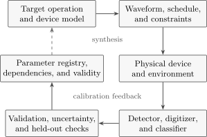
Reliable operation is cyclic. A model and parameter registry produce constrained waveforms; the device and environment produce detector records; inference and held-out validation determine whether parameters remain valid. Updates return through a dependency-aware calibration graph rather than silently changing unrelated operations.

The loop contains six distinct objects:

1. Target: a state, gate, channel, measurement, reset, transport operation, or logical cycle.
2. Model: Hamiltonians, dissipative terms, transfer functions, detector response, crosstalk, and parameter uncertainty.
3. Control program: waveforms, frequencies, phases, spatial patterns, pulse timing, switching, and feedforward rules.
4. Plant: the physical quantum device plus couplers, delivery lines, fields, optics, environment, and uncontrolled degrees of freedom.
5. Observation chain: transduction, amplification or photon collection, filtering, digitization, classification, timestamps, and metadata.
6. Update rule: parameter estimation, optimization, acceptance tests, validity intervals, and rollback.

Collapsing these objects creates ambiguity. A compiled pulse is not a gate until its action is characterized. An analog voltage at a digital-to-analog converter is not the field seen by a qubit. A classifier label is not the same object as the quantum measurement. A fitted optimum is not valid forever.

Layers and Timescales

Control systems operate on several coupled timescales:

Layer	Typical object	Update timescale	Failure if omitted
algorithm and logical schedule	gates, measurements, branches, syndrome rounds	per program or cycle	impossible timing or unsupported operations
compiler and pulse schedule	native gates, frame changes, routing, conflicts	per circuit or calibration epoch	unnecessary depth, collisions, or stale mappings
waveform synthesis	samples, phases, envelopes, chirps, switching	nanoseconds to milliseconds, platform dependent	wrong rotation, leakage, heating, or motion
detector and feedback	analog records, filters, classifier, decoder	within one shot or cycle	delayed reset, wrong branch, backlog
calibration	frequencies, amplitudes, transfer functions, thresholds	minutes to days, with faster tracking loops	systematic drift and invalid gates
health monitoring	loss, temperatures, laser lock, gain, noise, yield	continuous to scheduled	unrecognized regime change

The numerical times differ strongly across platforms. The architecture does not. Every layer needs a contract with the layer above and below, including timing, units, uncertainty, version, and validity.

From Commands to Physical Evolution

Controlled dynamics

A finite-dimensional model often begins with

$$H(t;\theta) = H_0(\theta) + \sum_{k=1}^{K} u_k(t)H_k(\theta),$$

where $\theta$ contains device parameters, $H_0$ is the drift Hamiltonian, $H_k$ are control generators, and $u_k(t)$ are physical fields or effective envelopes. For an open system, the corresponding model may be

$$\frac{d\rho}{dt} = -\frac{i}{\hbar}[H(t;\theta),\rho] + \mathcal D_{\theta,t}(\rho).$$

The control problem is not simply to choose any function $u_k(t)$. Real actuators impose:

• amplitude and energy bounds;
• finite bandwidth and sample rate;
• phase, frequency, and timing resolution;
• slew-rate and smoothness limits;
• finite spatial resolution and addressing spillover;
• shared-resource and simultaneous-operation constraints;
• heating, scattering, photon-number, or motional limits;
• waveform memory and streaming limits.

A pulse that is optimal for an unconstrained model but cannot be generated, delivered, synchronized, or calibrated is not an implementable control.

Reachability and native operations

The available generators determine which transformations are reachable and how costly they are. In closed finite-dimensional systems, Lie-algebraic controllability tests can establish whether combinations of $iH_0$ and $iH_k$ generate the desired unitary algebra. This is an existence statement. It does not determine a robust, short, low-leakage waveform under experimental constraints.

A “native gate” should therefore name:

• the physical interaction and frame;
• the calibrated pulse or parameterized family;
• duration and allowed parallel contexts;
• computational subspace and leakage treatment;
• phase convention and frame updates;
• validation protocol and expiration rule.

Virtual frame changes may have negligible physical duration, while still changing how every later pulse is interpreted. Their correctness depends on a shared phase reference and synchronized software state.

The Classical Delivery Chain

The requested digital envelope $u_{\mathrm{cmd}}(t)$ generally differs from the field at the device. In a linear time-invariant approximation,

$$u_{\mathrm{dev}}(t) = \int_{-\infty}^{\infty} h(t-t') u_{\mathrm{cmd}}(t')\,dt',$$

or, in frequency space,

$$U_{\mathrm{dev}}(\omega) = H(\omega)U_{\mathrm{cmd}}(\omega).$$

$H(\omega)$ includes digital filters, converters, mixers or modulators, cables, amplifiers, resonances, reflections, optical elements, and device coupling. Predistortion attempts to choose $U_{\mathrm{cmd}}$ so that the delivered field matches a target. Exact inversion is unsafe near zeros of $H(\omega)$ and can amplify noise, so regularization and amplitude constraints are required.

The linear model is only a starting point. Saturation, mixer imbalance, frequency-dependent phase, hysteresis, thermal effects, laser nonlinearities, ac Stark shifts, and state-dependent response can make the transfer context dependent.

Clock and reference integrity

Timing jitter, phase noise, frequency-reference drift, skew between channels, and trigger uncertainty can become quantum errors. A phase error $\delta\phi$ in a nominal equatorial qubit rotation changes its axis:

$$R_{\phi+\delta\phi}(\vartheta) \ne R_\phi(\vartheta).$$

Shared clocks reduce relative drift but can create common-mode correlated error. Independent references reduce some shared failure modes but require synchronization. The relevant specification follows from the quantum operation and circuit duration, not from a generic electronics data sheet.

Pulse Synthesis and Robustness

A control objective may minimize a cost

$$\begin{aligned} J[u] &= 1-F_{\mathrm{target}}[u] \\ &\quad + \lambda_E \sum_k \int_0^T \lvert u_k(t)\rvert^2\,dt \\ &\quad + \lambda_L L[u] + \lambda_S S[u], \end{aligned}$$

where $L[u]$ penalizes leakage and $S[u]$ penalizes bandwidth, roughness, sensitivity, or another engineering burden. The weights encode a design choice. A high simulated fidelity obtained by permitting excessive power or fragile spectral features may be inferior in the laboratory.

Gradient methods, Krotov updates, derivative-free search, analytic composite pulses, adiabatic methods, shortcut-to-adiabaticity ideas, and reinforcement-learning methods can all be useful. Their validity depends on model accuracy, constraints, measurement cost, and optimization landscape. The method name is not evidence of robustness.

Robust objectives

If uncertain parameters have distribution $\pi(\theta)$, an average robust objective is

$$\overline J[u] = \int J[u;\theta]\pi(\theta)\,d\theta.$$

A worst-case objective is

$$J_{\max}[u] = \max_{\theta\in\Theta} J[u;\theta].$$

Average robustness can tolerate rare poor regions; worst-case robustness can be conservative and expensive. State which uncertainty set or distribution was used and validate on held-out parameter values.

Leakage-aware shaping

Fast driving of a weakly anharmonic system can populate levels outside the computational subspace. Derivative-based quadrature corrections, spectral shaping, longer pulses, and optimal control can reduce leakage, but they require calibration of anharmonicity, transfer functions, and frame phases. Suppressing final leakage does not guarantee that transient leakage is harmless: population outside the code space can acquire phases or interact with spectators during the pulse.

Calibration Is Statistical Inference

A calibration experiment chooses settings $x$, observes data $D$, and estimates parameters $\theta$ through a model

$$p(D\mid x,\theta).$$

The output is not merely “the best knob value.” It should include uncertainty, goodness-of-fit, validity conditions, and downstream dependencies.

Examples include:

• transition or resonance frequency;
• Rabi rate versus amplitude;
• phase offsets and frame alignment;
• entangling-interaction strength and conditional phase;
• pulse-transfer function and channel delay;
• readout weights, thresholds, and confusion matrix;
• crosstalk coefficients and simultaneous-operation corrections;
• reset parameters and residual population;
• drift model and recalibration trigger.

Quantum Measurement as Estimation owns likelihood, estimator, loss, bias, variance, and uncertainty. Calibration applies that contract to the control stack.

Calibration dependencies

Calibrations form a directed graph. A readout threshold may depend on resonance frequency and gain. A $\pi$-pulse amplitude may depend on drive frequency, transfer function, and pulse duration. An entangling gate may depend on both one-qubit frames and coupler bias. If an upstream parameter changes, downstream calibrations may become stale.

For a dependency graph $G_{\mathrm{cal}}=(V,E)$, an edge

$$a\longrightarrow b$$

means calibration $b$ assumes a valid result from $a$. A directed acyclic portion can be updated in topological order. Real systems may contain loops, such as readout needed to calibrate control while control is needed to prepare readout references. Those loops require bootstrapping, joint estimation, or progressively refined procedures.

The registry for each calibration should store:

• value, units, uncertainty, and covariance where relevant;
• device, channel, and operating context;
• parent calibrations and versions;
• acquisition data and fit code version;
• acceptance criteria and validation result;
• timestamp, expiration, and health indicators;
• previous valid value and rollback path.

This establishes the physical dependency principle. Calibration Loops develops the canonical record schema, impact-aware invalidation, graph and resource scheduling, candidate acceptance, and atomic update protocol.

Open-loop, closed-loop, and adaptive calibration

Model-based open-loop control computes a waveform from an estimated model and executes it without measuring during the operation. It can still be recalibrated between experiments.

Closed-loop calibration evaluates an outcome and updates control parameters over repeated trials. The feedback acts on future experiments, not necessarily within one quantum trajectory.

Real-time measurement feedback uses a record from the current shot to choose a later operation in that same shot.

These loops have different latency and disturbance requirements. Calling all of them “feedback” without a timescale is ambiguous.

Two Basic Tune-Up Experiments

Rabi amplitude calibration

For a resonantly driven ideal two-level system initially in $\lvert0\rangle$,

$$P_1(t) = \sin^2 \left( \frac{\Omega t}{2} \right).$$

A nominal $\pi$ pulse satisfies

$$t_\pi = \frac{\pi}{\Omega}.$$

In practice, fit contrast, offset, damping, detuning, and possibly leakage. A Rabi scan estimates an amplitude-times-duration relation at one operating point. It does not by itself calibrate phase, simultaneous context, or long-sequence coherent accumulation.

Ramsey frequency and frame calibration

Two nominal $\pi/2$ pulses separated by delay $\tau$ can produce

$$P_1(\tau) = B + A e^{-(\tau/T_2^\ast)^\beta} \cos(\Delta\omega\,\tau+\phi).$$

The fitted detuning $\Delta\omega$ updates a drive frequency or software frame. The phase $\phi$ can reveal timing or reference offsets. A frequency estimate should be validated at later times and across the pulse contexts in which it will be used.

Calibration is not validation

If the same Rabi or Ramsey data choose parameters and certify the resulting gate, the reported performance is in-sample. A stronger workflow freezes the calibration and tests held-out sequences, amplitudes, delays, states, and simultaneous contexts. Randomized benchmarking, cycle benchmarking, tomography, or application-specific checks can then validate consequences not explicitly fitted.

Dynamical Decoupling owns compiled control-window eligibility, protected estimands, total-cost accounting, and held-out deployment decisions; this page retains pulse calibration, physical delivery, leakage and crosstalk measurement, and epoch-bound validity evidence.

Initialization and Reset

State preparation removes entropy and establishes the input contract. Common methods include:

• passive relaxation or optical pumping;
• active coherent transfer;
• measurement and conditional correction;
• heralded preparation with explicit success probability;
• engineered dissipation or reservoir stabilization;
• cooling of motion or auxiliary modes;
• loading, rearrangement, and replacement of physical carriers.

Reset should be reported as a channel with duration, residual error, leakage or loss, and effect on neighboring systems. A heralded reset with excellent conditional fidelity may have poor throughput if success is rare. A fast reset can introduce correlated heating or photons that disturb subsequent operations.

For repeated circuits and error correction, reset must also integrate with scheduling: when the classical result arrives, when the correction begins, and whether another ancilla can be prepared in parallel.

The Readout Chain

Readout has a quantum stage and a classical stage.

1. A system observable couples to a pointer degree of freedom.
2. The pointer modifies a field, fluorescence pattern, charge state, current, phase, arrival time, or detector event.
3. The signal propagates through collection, amplification, filtering, or conversion.
4. An analog-to-digital or event-timing system records data.
5. A filter or inference model maps the record to an outcome and confidence.
6. A quantum instrument assigns both outcome probability and conditional state update.

The classical label is only the end of the chain.

Filtered records and classifiers

Let $y(t)$ be a real or complex detector record. A linear statistic can be

$$z = \int_0^{T_m} w^\dagger(t)y(t)\,dt,$$

where $w(t)$ is a matched or otherwise chosen filter. A threshold or multiclass rule maps $z$ to an outcome. When the noise is Gaussian with known class means and covariance, a likelihood-ratio classifier can be optimal for the assumed model. Relaxation during measurement, nonstationary noise, overlapping events, and hidden leakage can require nonlinear filters or temporal models.

Training and test data must be separated. Continually adjusting a threshold on the same records used to report assignment fidelity biases the estimate.

POVMs and instruments

The detector outcomes are represented by a POVM $\{M_m\}$:

$$p(m\mid\rho) = \operatorname{Tr}(M_m\rho).$$

The state update is represented by a quantum instrument $\{\mathcal I_m\}$:

$$\widetilde\rho_m = \mathcal I_m(\rho), \qquad p(m\mid\rho) = \operatorname{Tr}\widetilde\rho_m.$$

Two detectors can have similar assignment matrices but different backaction. That distinction matters for repeated syndrome extraction, adaptive circuits, and state reuse. Quantum Instruments owns the full formalism, while Measurement Tomography explains how effects can be reconstructed.

SPAM Errors owns the operational preparation–measurement composition, assignment and confusion distinction, identifiability, gauge, context-transfer tests, and mitigation licenses. Measurement Error Mitigation owns subsequent terminal-response correction and its inverse or forward estimators, constraints, regularization, science and calibration covariance, structured scaling, and drift-qualified validation; this page retains physical initialization, reset, detector-chain, classifier, backaction, feedback, and calibration engineering. Zero-Noise Extrapolation owns folding, stretching, and probabilistic amplification as calibrated scaling experiments together with coordinate-zero intercept inference; this page retains waveform, inverse-gate, scheduling, readout, feedback, and recalibration engineering.

Quantum non-demolition behavior

A measurement is quantum non-demolition relative to an observable when repeated measurement can reveal that observable without the measurement dynamics causing transitions between its eigenspaces, under the stated model. Practical tests should separate:

• first-readout assignment error;
• conditional state disturbance;
• relaxation or excitation between readouts;
• leakage and loss;
• correlated detector memory.

High agreement between repeated labels can arise from a detector bias and is therefore not sufficient alone.

Multiplexing and readout crosstalk

Multiplexing shares detectors, frequency bands, optical paths, cameras, amplifiers, or digitizers. It reduces hardware fan-out but introduces dynamic-range, spectral-collision, bandwidth, and classifier-correlation constraints. Compare isolated and simultaneous readout, including spectator dephasing and measurement-induced transitions.

The full confusion matrix can grow exponentially with qubit count, so scalable models often assume locality or low-order correlations. Those assumptions should be tested rather than treated as definitions.

Real-Time Feedback and Feedforward

If outcome $m$ selects a conditional operation $\mathcal C_m$, the unconditional feedback channel is

$$\mathcal E_{\mathrm{fb}}(\rho) = \sum_m \mathcal C_m \circ \mathcal I_m(\rho).$$

This form makes clear that feedback includes measurement backaction and classical branching. It is not equivalent to applying a unitary to an unmeasured state.

The latency budget may be decomposed as

$$\begin{aligned} t_{\mathrm{fb}} &= t_{\mathrm{interact}} + t_{\mathrm{propagate}} + t_{\mathrm{digitize}} \\ &\quad + t_{\mathrm{infer}} + t_{\mathrm{decide}} + t_{\mathrm{actuate}}. \end{aligned}$$

The state continues to evolve during this delay. A feedback protocol must include idle evolution, decoherence, and frame accumulation between measurement and correction.

Feedforward often means that an earlier known result changes a later control without attempting to stabilize a continuously monitored state. Feedback emphasizes regulation using observed deviations. The distinction is contextual; the data dependency and latency are more important than the label.

Measurement-Based Feedback and Feedback from Records own the stochastic state-estimation theory.

Mid-Circuit Measurement and Feedforward owns the ideal logical dependency graph, branch maps, reset and reuse contract, and abstract branch costs. This page retains detector, classifier, controller, actuation, calibrated duration and jitter, and evolution-during-delay evidence.

Crosstalk and Simultaneous Control

For small classical cross-coupling, delivered controls may be approximated by

$$\mathbf u_{\mathrm{dev}}(\omega) = H(\omega)\mathbf u_{\mathrm{cmd}}(\omega),$$

where off-diagonal entries of $H$ represent channel crosstalk. Predistortion can compensate a stable, identified matrix over a limited bandwidth. It cannot remove state-dependent interactions, heating, shared quantum modes, detector backaction, or unmodeled nonlinearities.

Simultaneous calibration should probe:

• neighboring and distant spectator states;
• overlapping gates and measurements;
• power and duty-cycle dependence;
• frequency and timing collisions;
• correlated residuals rather than only marginal errors;
• context changes caused by routing or compiler schedules.

An isolated calibration table is not sufficient evidence for a parallel processor.

Drift, Monitoring, and Recalibration

Let $\theta(t)$ be a calibrated parameter and $\widehat\theta(t_j)$ periodic estimates. A policy needs:

• a health statistic or residual;
• warning and invalidation thresholds;
• sampling cadence;
• dependence on temperature, loading, gain, or other telemetry;
• action on a warning;
• rollback and data provenance.

A fixed calendar interval is simple but can recalibrate too often during stable periods and too late during abrupt change. Event-triggered policies use health checks or change-point detection, but must control false alarms and missed changes.

Calibration can itself disturb operation. It consumes shots, changes bias or power, and may invalidate neighboring parameters. Scheduling calibration is therefore an experimental-design and operations problem, not merely a curve fit.

Calibration Loops gives the detailed supervisory treatment of latent-state tracking, change triggers, hysteresis, loop stability, prioritization, and failure recovery.

Safe updates

An updated parameter should pass:

1. fit and identifiability checks;
2. physical bounds and consistency checks;
3. a local held-out validation;
4. a simultaneous-context validation when relevant;
5. comparison against the incumbent value;
6. rollback criteria.

Blindly accepting every numerical optimizer output can turn statistical fluctuation into control drift.

Scaling the Stack

Scaling the quantum device changes the classical system:

• more waveform and detector channels require fan-out or multiplexing;
• synchronization and clock distribution become network problems;
• calibration dependencies grow and need automated scheduling;
• raw readout bandwidth can exceed central data links;
• feedback and decoding require distributed low-latency computation;
• parameter storage, provenance, and reproducibility become database problems;
• thermal, optical, electrical, and mechanical resources constrain duty cycle;
• failure isolation and degraded modes become necessary for availability.

Parallelism is central. If each of $N$ qubits requires a serial calibration taking time $\tau$, naive calibration takes $N\tau$. Locality and graph coloring may permit independent calibrations in parallel, but only after crosstalk constraints are measured.

For quantum error correction, the classical processor must sustain the syndrome stream. If each round produces $B$ bits every $t_{\mathrm{round}}$, the raw rate is

$$R_{\mathrm{syn}} = \frac{B}{t_{\mathrm{round}}}.$$

Throughput above this rate is necessary but not sufficient. Tail latency, memory, communication, decoder accuracy, and conditional-control deadlines also matter. Decoders develops those QEC-specific inference and timing requirements.

Platform Manifestations

The loop is shared; its physical implementation is not.

Platform	Control carrier	Representative readout	Calibration pressure
superconducting circuits	microwave envelopes, flux bias, tunable couplers	dispersive microwave field and amplifier chain	frequency crowding, transfer distortion, leakage, cryogenic and simultaneous crosstalk
trapped ions	laser or microwave amplitude, phase, frequency, and trap waveforms	state-dependent fluorescence	optical phase, motional modes, beam alignment, intensity, magnetic-field drift
neutral atoms	tweezer patterns, microwave and optical fields, Rydberg pulses	fluorescence imaging and loss detection	loading, rearrangement, spatial inhomogeneity, motion, laser detuning and intensity
photonics	source pumps, phase shifters, switches, delays, feedforward	photon counting or homodyne and heterodyne records	loss, indistinguishability, interferometer phase, detector timing, source synchronization
semiconductor spins	voltage pulses, exchange, microwave magnetic or electric drive	spin-to-charge conversion and charge sensing	device variability, cross-capacitance, charge noise, dense cryogenic wiring
solid-state defects	microwave and optical fields	spin-dependent fluorescence or optical transition	spectral diffusion, charge state, collection, local strain and field
bosonic and continuous-variable modes	displacements, squeezing, parametric drives, ancilla controls	parity mapping, homodyne, heterodyne, or photon counting	phase-space calibration, finite squeezing, ancilla errors, mode selectivity

The platform pages own the specific encodings and apparatus. This page owns the common systems contract.

Worked End-to-End Example

Consider an ideal qubit driven on resonance with observed Rabi frequency

$$f_R = 10\,\mathrm{MHz}.$$

Since $\Omega=2\pi f_R$, a $\pi$ pulse has duration

$$t_\pi = \frac{\pi}{2\pi f_R} = \frac{1}{2f_R} = 50\,\mathrm{ns}.$$

A Ramsey fit then finds drive detuning

$$\frac{\Delta\omega}{2\pi} = 200\,\mathrm{kHz}.$$

The controller can update the oscillator frequency or accumulate a software frame correction

$$\Delta\phi(t) = \Delta\omega\,t.$$

Neither update is accepted solely because it improves the calibration fit. A held-out long-sequence test checks phase accumulation and a simultaneous test checks spectator effects.

Suppose the readout statistic is Gaussian with equal variance:

$$\begin{aligned} z\mid0 &\sim \mathcal N(-1,0.5^2), \\ z\mid1 &\sim \mathcal N(1,0.5^2). \end{aligned}$$

With equal prior probabilities and threshold $z=0$, each idealized assignment error is

$$\Phi(-2) \approx 0.0228,$$

so the mean assignment fidelity is about $97.7\%$. This calculation assumes stationary Gaussian distributions and no relaxation, leakage, or drift. Those assumptions are tested on held-out records.

Finally, let the measured feedback stages be

$$\begin{aligned} t_{\mathrm{int+prop}} &=200\,\mathrm{ns}, \\ t_{\mathrm{dig+infer}} &=70\,\mathrm{ns}, \\ t_{\mathrm{decide+trigger}} &=80\,\mathrm{ns}, \\ t_{\mathrm{actuate}} &=50\,\mathrm{ns}. \end{aligned}$$

The total is

$$t_{\mathrm{fb}} = 400\,\mathrm{ns}.$$

A feedback simulation must evolve the state through that delay. Quoting only the $70\,\mathrm{ns}$ classifier time would misstate the physical loop.

Common Mistakes

• Equating a digital waveform with the delivered field. Transfer functions, clocks, nonlinearities, and crosstalk intervene.
• Calling a simulated optimum calibrated. Model error and experimental constraints require closed-loop validation.
• Using calibration data as independent validation data. In-sample fit quality overstates predictive evidence.
• Changing an upstream parameter without invalidating dependents. Calibration values form a graph, not a flat table.
• Optimizing one gate in isolation and inferring parallel performance. Simultaneous controls change the plant.
• Reporting a classifier accuracy as the complete measurement. Backaction, loss, latency, and conditional state matter.
• Calling repeated-label agreement quantum non-demolition fidelity. Detector bias and between-readout dynamics must be separated.
• Omitting rejected events. Conditional fidelity must be paired with unconditional success and throughput.
• Ignoring the state evolution during feedback latency. The correction acts on a later state.
• Treating reset fidelity without reset time. Repetition rate and ancilla supply depend on both.
• Recalibrating on every fluctuation. Noisy parameter updates can make control less stable.
• Storing values without units, provenance, or validity. Reproducibility then depends on undocumented operator knowledge.

Exercises

1. Calibrate a π pulse

An ideal resonant Rabi experiment gives $f_R=8\,\mathrm{MHz}$. Find the $\pi$-pulse and $\pi/2$-pulse durations.

Solution

For $P_1(t)=\sin^2(\pi f_R t)$,

$$t_\pi = \frac{1}{2f_R} = \frac{1}{16\,\mathrm{MHz}} = 62.5\,\mathrm{ns}.$$

The $\pi/2$ pulse has half that duration:

$$t_{\pi/2} = 31.25\,\mathrm{ns}.$$

This conversion assumes amplitude scales linearly, the drive is resonant, and pulse edges or transfer distortion do not alter the effective rotation.

2. Update a Ramsey frame

A Ramsey fit finds $\Delta f=25\,\mathrm{kHz}$. What phase error accumulates in $40\,\mu\mathrm{s}$?

Solution

$$\begin{aligned} \Delta\phi &= 2\pi\Delta f\,t \\ &= 2\pi (25\times10^3) (40\times10^{-6}) \\ &= 2\pi. \end{aligned}$$

The phase error is one full cycle. Although the final angle is equivalent modulo $2\pi$ at exactly this delay, intermediate gates and nearby delays are affected. The controller should correct the frequency or track the frame continuously.

3. Propagate a pure delay

A delivery line has transfer function

$$H(\omega) = e^{-i\omega\tau}$$

with $\tau=12\,\mathrm{ns}$. What time-domain effect does it produce, and how should a synchronized schedule compensate it?

Solution

The inverse transform gives a delayed waveform:

$$u_{\mathrm{dev}}(t) = u_{\mathrm{cmd}}(t-\tau).$$

The controller can launch that channel $12\,\mathrm{ns}$ earlier relative to a common device-time reference. Compensation must include every channel’s delay; advancing one waveform without updating triggers and phase references can create a different timing error.

4. Regularize an inverse filter

Why is the formal predistortion

$$U_{\mathrm{cmd}}(\omega) = \frac{U_{\mathrm{target}}(\omega)} {H(\omega)}$$

unsafe when $\lvert H(\omega)\rvert$ is very small?

Solution

Division by a small transfer magnitude produces a very large command amplitude and amplifies measurement noise and modeling error. The requested signal may violate actuator limits or excite unmodeled dynamics. A practical inverse limits bandwidth, penalizes command power, or uses a regularized factor such as

$$\frac{H^\ast(\omega)} {\lvert H(\omega)\rvert^2+\lambda}.$$

The achieved device waveform and gate must then be validated experimentally.

5. Choose a Gaussian readout threshold

Two equally likely readout classes have

$$\begin{aligned} z\mid0 &\sim \mathcal N(-0.8,0.4^2), \\ z\mid1 &\sim \mathcal N(0.8,0.4^2). \end{aligned}$$

Find the symmetric threshold and the error probability for each class.

Solution

Equal priors and equal variances place the likelihood-ratio threshold midway at $z=0$. For class $0$,

$$\begin{aligned} p(1\mid0) &= 1-\Phi \left( \frac{0-(-0.8)}{0.4} \right) \\ &= 1-\Phi(2). \end{aligned}$$

For class $1$,

$$p(0\mid1) = \Phi(-2).$$

Both are approximately $0.0228$, giving idealized mean assignment fidelity $0.9772$.

6. Separate assignment and backaction

A detector reports the correct prepared label $99\%$ of the time, but after outcome $0$ the system is found in the corresponding eigenspace only $94\%$ of the time. Which two properties have been measured?

Solution

The first number is a state-preparation-and-assignment property for the tested reference states. The second probes conditional state preservation or quantum non-demolition behavior after outcome $0$. High assignment accuracy does not imply low backaction, so both numbers are needed for repeated measurement or feedback.

7. Compute feedback latency

A readout interaction takes $300\,\mathrm{ns}$, signal propagation $40\,\mathrm{ns}$, digitization and filtering $90\,\mathrm{ns}$, decision logic $30\,\mathrm{ns}$, and actuator response $60\,\mathrm{ns}$. Find the closed-loop latency.

Solution

With no overlap,

$$\begin{aligned} t_{\mathrm{fb}} &= 300+40+90+30+60 \\ &= 520\,\mathrm{ns}. \end{aligned}$$

If stages overlap, the schedule should use their actual dependency graph rather than this sum. The quantum state must be propagated for the implemented latency.

8. Order a calibration graph

Calibration $A$ finds readout resonance, $B$ finds a readout classifier, $C$ finds drive frequency, and $D$ finds a $\pi$-pulse amplitude. Suppose $B$ depends on $A$, while $D$ depends on $B$ and $C$. Give valid update orders.

Solution

$A$ must precede $B$, and both $B$ and $C$ must precede $D$. Valid orders include

$$A,\ B,\ C,\ D$$

and

$$C,\ A,\ B,\ D.$$

$A$ and $C$ are independent under the declared graph and may run in parallel. If updating $C$ changes the readout response, the graph is incomplete and must add that dependency.

9. Compare average and worst-case robust control

Two uncertain parameter values have costs $J_1=10^{-4}$ and $J_2=10^{-2}$ with probabilities $0.99$ and $0.01$. Compute the average cost and worst-case cost.

Solution

$$\begin{aligned} \overline J &= 0.99(10^{-4}) + 0.01(10^{-2}) \\ &= 1.99\times10^{-4}. \end{aligned}$$

The worst-case cost is

$$J_{\max} = 10^{-2}.$$

The average objective regards the poor region as rare; the worst-case objective does not. The appropriate choice depends on whether rare excursions can be detected, tolerated, or made safe.

10. Design a held-out validation

A pulse amplitude and readout threshold were tuned by minimizing assignment error on repeated $\lvert0\rangle$ and $\lvert1\rangle$ preparations. Propose a held-out validation that tests more than fit quality.

Solution

Freeze both parameters. Acquire new time-interleaved data not used in tuning, including $\lvert0\rangle$, $\lvert1\rangle$, superposition preparations, repeated readout, and simultaneous activity on selected spectators. Predeclare assignment, leakage, conditional-state, and crosstalk metrics with confidence intervals. The new data test generalization; superpositions and repeated readout probe backaction; spectators test context. Retuning after viewing the held-out data begins a new calibration epoch and requires another validation set.

References

1. S. J. Glaser et al., “Training Schrödinger’s cat: Quantum optimal control,” European Physical Journal D 69, 279 (2015), doi:10.1140/epjd/e2015-60464-1.
2. C. P. Koch et al., “Quantum optimal control in quantum technologies: Strategic report on current status, visions and goals,” EPJ Quantum Technology 9, 19 (2022), doi:10.1140/epjqt/s40507-022-00138-x.
3. N. Khaneja, T. Reiss, C. Kehlet, T. Schulte-Herbrüggen, and S. J. Glaser, “Optimal control of coupled spin dynamics: Design of NMR pulse sequences by gradient ascent algorithms,” Journal of Magnetic Resonance 172, 296–305 (2005), doi:10.1016/j.jmr.2004.11.004.
4. J. P. Palao and R. Kosloff, “Quantum computing by an optimal control algorithm for unitary transformations,” Physical Review Letters 89, 188301 (2002), doi:10.1103/PhysRevLett.89.188301.
5. F. Motzoi, J. M. Gambetta, P. Rebentrost, and F. K. Wilhelm, “Simple pulses for elimination of leakage in weakly nonlinear qubits,” Physical Review Letters 103, 110501 (2009), doi:10.1103/PhysRevLett.103.110501.
6. J. Kelly et al., “Scalable in situ qubit calibration during repetitive error detection,” Physical Review A 94, 032321 (2016), doi:10.1103/PhysRevA.94.032321.
7. J. Kelly, P. O’Malley, M. Neeley, H. Neven, and J. M. Martinis, “Physical qubit calibration on a directed acyclic graph,” arXiv:1803.03226 (2018), arXiv:1803.03226.
8. J. Gambetta, W. A. Braff, A. Wallraff, S. M. Girvin, and R. J. Schoelkopf, “Protocols for optimal readout of qubits using a continuous quantum nondemolition measurement,” Physical Review A 76, 012325 (2007), doi:10.1103/PhysRevA.76.012325.
9. J. Heinsoo et al., “Rapid high-fidelity multiplexed readout of superconducting qubits,” Physical Review Applied 10, 034040 (2018), doi:10.1103/PhysRevApplied.10.034040.
10. D. Ristè, C. C. Bultink, K. W. Lehnert, and L. DiCarlo, “Feedback control of a solid-state qubit using high-fidelity projective measurement,” Physical Review Letters 109, 240502 (2012), doi:10.1103/PhysRevLett.109.240502.
11. R. Vijay et al., “Stabilizing Rabi oscillations in a superconducting qubit using quantum feedback,” Nature 490, 77–80 (2012), doi:10.1038/nature11505.
12. P. Campagne-Ibarcq et al., “Persistent control of a superconducting qubit by stroboscopic measurement feedback,” Physical Review X 3, 021008 (2013), doi:10.1103/PhysRevX.3.021008.
13. J. Zhang, Y. Liu, R. Wu, K. Jacobs, and F. Nori, “Quantum feedback: Theory, experiments, and applications,” Physics Reports 679, 1–60 (2017), doi:10.1016/j.physrep.2017.02.003.
14. L. Bouten, R. van Handel, and M. R. James, “An introduction to quantum filtering,” SIAM Journal on Control and Optimization 46, 2199–2241 (2007), doi:10.1137/060651239.
15. J. P. G. van Dijk et al., “Impact of classical control electronics on qubit fidelity,” Physical Review Applied 12, 044054 (2019), doi:10.1103/PhysRevApplied.12.044054.
16. P. Krantz et al., “A quantum engineer’s guide to superconducting qubits,” Applied Physics Reviews 6, 021318 (2019), doi:10.1063/1.5089550.
17. A. Blais, A. L. Grimsmo, S. M. Girvin, and A. Wallraff, “Circuit quantum electrodynamics,” Reviews of Modern Physics 93, 025005 (2021), doi:10.1103/RevModPhys.93.025005.
18. C. D. Bruzewicz, J. Chiaverini, R. McConnell, and J. M. Sage, “Trapped-ion quantum computing: Progress and challenges,” Applied Physics Reviews 6, 021314 (2019), doi:10.1063/1.5088164.
19. M. Saffman, “Quantum computing with atomic qubits and Rydberg interactions: Progress and challenges,” Journal of Physics B 49, 202001 (2016), doi:10.1088/0953-4075/49/20/202001.
20. J. E. Gough, “Principles and applications of quantum control engineering,” Philosophical Transactions of the Royal Society A 370, 5239–5240 (2012), doi:10.1098/rsta.2012.0331.

Further Connections

• Hardware Overview places this loop inside the full physical-to-logical architecture.
• Quantum Software Stack owns the boundary between target-specific lowering, dispatched controller artifacts, runtime records, and reproducible postprocessing.
• Circuit Intermediate Representations defines the profile, timing, units, result schema, and target-state contracts a controller-facing IR must make explicit.
• Error-Aware Compilation explains how a compiler consumes dated estimates, uncertainty, crosstalk context, and validity intervals without treating calibration as timeless truth.
• Pulse-Level Control owns the software-to-controller contract for frames, waveform materialization, sampling, scheduling, transfer-model bindings, and pulse certificates.
• Calibration Loops owns dependency-aware maintenance, drift triggers, held-out candidate acceptance, atomic publication, rollback, and quarantine.
• Device Characterization develops the inverse problem that turns spectroscopy, control, and readout records into identifiable, uncertainty-qualified, predictively tested device models.
• Metrics for Quantum Hardware defines the estimands and uncertainty statements used to accept or reject calibrations.
• Modular Architectures extends the control loop across module clocks, heralds, routing, resource inventory, feed-forward, decoder state, and shared fault domains.
• Superconducting Qubits instantiates this loop with microwave and flux control, dispersive readout, tunable couplers, frequency allocation, and cryogenic routing.
• Optimal Control develops gradients, control landscapes, constraints, and open-system objectives.
• Optimal Control for Quantum Processors compares deployable optimization regimes and separates optimizer scores, hardware refinement, qualification, and release.
• Rabi and Ramsey Control owns the driven two-level dynamics behind the basic tune-up experiments.
• Pulse Sequences and Dynamical Decoupling develop composite timing and filter-function ideas.
• Quantum Instruments separates outcome probabilities from conditional state updates.
• Input–Output Theory connects internal modes to propagating fields and detector records.
• Feedback from Records develops filtering, innovations, delayed control, and stochastic feedback.
• Noise in Quantum Information classifies the drift, leakage, crosstalk, correlation, and model mismatch that calibration must expose.