SPAM Errors

State-preparation and measurement (SPAM) errors live at different boundaries of an experiment. What the laboratory directly supplies is a probability table for declared commands, circuits, settings, contexts, and times—not a unique allocation of its discrepancies to an initial state and a final detector. A column-stochastic assignment matrix is useful only for a restricted, basis-diagonal terminal response. This page builds the broader operational record: preparation states and operations, POVMs and instruments, empirical confusion tables, nonidentifiability and gauge, context and drift tests, and the evidence needed to license characterization, transfer, or estimand-specific mitigation.

Required background. Measurement in Circuits supplies the ideal outcome, record, bit-order, and circuit-location conventions used here. Quantum Instruments supplies the distinction between outcome effects and conditional state updates.

Helpful background. Quantum Channels for QI fixes composition and representation conventions, while Variance and Covariance supplies the covariance propagation used for corrected estimators.

SPAM Is a Boundary Model, Not One Error Rate

Preparation and measurement occupy different boundaries

A preparation command $x$ acts before the declared process. Its actual output may be a density operator, a correlated system–environment state, or a branch of a preparation instrument carrying a reset or heralding record. A measurement setting $s$ acts after that process. Its outcome probabilities are described by effects, while its conditional output and disturbance require an instrument. Moving either discrepancy to the other boundary changes the physical claim unless an explicit model or gauge transformation licenses that reassignment.

This separation matters even when only one scalar is reported. A wrong initial population, coherent preparation phase, detector threshold error, and measurement-induced transition can produce the same basis-state frequency in one circuit but make different predictions after an intervening rotation or a repeated readout. The broad mechanism taxonomy belongs to Noise in Quantum Information; here the concern is which boundary object and inference are licensed by the data.

Error requires a target and trusted boundary

An error is a discrepancy from a declared target. A preparation claim therefore names an intended state or operation and the point in the circuit where it should exist. A measurement claim names ideal effects, an ideal instrument, or a classical record map and the time at which it is compared. Changing the target basis, accepted sector, or reporting alphabet can change the numerical error without changing the apparatus.

The target defines the mathematical discrepancy; trust or independently justified bounds make its experimental attribution possible. For example, state infidelity is well defined once $\rho_x$ and $\rho_x^{\rm tar}$ are specified, but inferring it from frequencies requires a calibrated or bounded measurement model. Conversely, detector tomography needs trusted probe states or a self-consistent design with its unresolved freedoms exposed. “Trusted” is thus a causal and stability assumption about an experimental boundary, not a compliment to a component.

A scalar cannot carry a SPAM model

One number cannot preserve dependence on input state, measurement basis, outcome asymmetry, conditional backaction, leakage, invalid records, multiqubit correlations, acceptance, context, or epoch. Even the common average assignment fidelity compresses two conditional error probabilities and says nothing about off-diagonal POVM components. A scalar may be a useful estimand after its preparation ensemble, weights, loss policy, and validity window are fixed; it is not a portable model of the boundary.

The minimum defensible report therefore pairs every scalar with its target, forward model, acquisition design, uncertainty, and falsifiers. If later work needs a different state ensemble, simultaneous schedule, or repeated-measurement behavior, it must return to the richer record rather than silently reusing the scalar.

Freeze the Preparation–Process–Measurement Record

Labels, spaces, bases, and record codes

Fix the physical system, encoded sector, any leakage or loss sector, and the input and output Hilbert spaces of every operation. Give preparation commands $x$ , retained preparation records $r$ , measurement settings $s$ , latent ideal outcomes $z$ , and reported outcomes $y$ distinct symbols. Specify the ideal basis $\{\Pi_z\}$ , tensor order, bitstring order, endianness, and whether a reported string names physical wires or classical registers.

The outcome alphabet must include every event used in the likelihood. An erasure, leakage flag, timeout, saturation event, or invalid classifier code is not automatically an ordinary bit. Coarse graining is a declared classical map applied after data acquisition; it is not permission to erase the frequency of discarded events. The retained sector and alphabet determine which normalization statements are valid.

Circuit location, context, epoch, and acquisition order

Place preparation, the intervening sequence $\mathbf g$ , and measurement at explicit circuit locations. Record spectator states, simultaneous drives and readouts, reset history, integration windows, classifier versions, feedback, and any accepted branch. Attach timestamps or epochs $t$ and contexts $c$ . A response calibrated in isolation at one epoch is not, by notation alone, the response during a simultaneous circuit later that day.

Acquisition order is part of the design. Blocks of all calibration shots followed by all science shots can confound drift with command dependence. Randomized or rastered ordering, interleaved references, and retained timestamps allow that alternative to be tested. Randomization does not make a drifting device stationary; it changes which averages are estimable and makes some confounding visible.

Acceptance, estimand, and evidence

The following record prevents a “SPAM rate” from changing meaning between calibration, validation, and use.

Record field	What must be frozen
System, encoding, retained sectors, and trusted boundary	Physical carriers, computational and enlarged spaces, accepted sectors, and which boundary is treated as known or bounded.
Nominal preparation commands, target states, and reference input	Command labels, target density operators or maps, reference state, basis, phases, and preparation ensemble weights.
Actual preparation operations, heralding, reset history, and acceptance	CP branches, retained records, success probabilities, rejected outcomes, reset mode, and state carried between shots.
Intervening process, circuit, location, and schedule	Ordered gates or channels, delays, circuit placement, simultaneous activity, feedback, and whether the process is unconditional or selected.
Measurement settings, effects, instrument, and output space	Setting labels, POVM effects, conditional maps, measured subsystem, postmeasurement space, and repeated-use claim.
Classical codes, bit order, invalid outcomes, and coarse graining	Report alphabet, wire-to-bit map, string order, analog-to-digital rule, invalid-code frequency, and every merge or discard rule.
Context, spectators, history, epoch, and acquisition order	Remote states and operations, previous outcomes, classifier version, timestamps, blocks, randomization, and change points.
Data, trusted references, identifiability, gauge, and model family	Counts or records, trusted or bounded objects, observable parameter combinations, remaining coordinate freedom, and alternatives tested.
Estimand, metrics, uncertainty, holdouts, and falsifiers	Exact quantity reported, weighting, confidence or credible procedure, reserved data, sensitivity, and rejection criterion.
Characterization or mitigation action, cost, validity window, and owner	Downstream decision, calibration and shot cost, transfer domain, expiry rule, provenance, and canonical specialist page.

Acceptance probability is part of the estimand, not nuisance metadata. A postselected conditional mean answers a different question from an unconditional device yield. Likewise, a fitted parameter, a held-out predictive score, and a mitigated observable are different outputs and require separate uncertainty and validity statements.

Preparation States, Maps, and Heralded Branches

Actual emitted states and replacement maps

For command $x$ , record $r$ , epoch $t$ , and context $c$ , a preparation instrument has completely positive, trace-nonincreasing branches $\mathcal P_{r|x,t,c}$ whose sum is trace preserving. Acting on a declared reference input gives a subnormalized output

\widetilde\rho_{r|x,t,c} = \mathcal P_{r|x,t,c}(\sigma_{\rm ref}), \qquad \sum_r\mathcal P_{r|x,t,c} \ \text{is trace preserving}.

Its trace is the branch probability. When the apparatus simply emits a normalized state $\rho_x$ and no meaningful quantum input is retained, the replacement channel

\mathcal R_{\rho_x}(X) = \operatorname{Tr}(X)\rho_x

is a convenient operational representation. If $\rho_x=\sum_a\lambda_a|a\rangle\langle a|$ and $\{|j\rangle\}$ is an input basis, Kraus operators $K_{aj}=\sqrt{\lambda_a}|a\rangle\langle j|$ give the map and satisfy $\sum_{a,j}K_{aj}^{\dagger}K_{aj}=I$ . Positivity of $\rho_x$ gives complete positivity and $\operatorname{Tr}\rho_x=1$ gives trace preservation. This representation fixes the emitted state, not a unique reset, cooling, pulse, or thermalization mechanism.

Target-relative state metrics

For a pure target $|\psi_x\rangle$ , a common preparation infidelity is

r_x^{\rm prep} = 1-\langle\psi_x|\rho_x|\psi_x\rangle.

For mixed targets one must state the fidelity convention and whether “fidelity” is squared. Such a metric can distinguish neither a coherent axis error from a mixture nor a reset failure from a correlated spectator without additional probes. Ensemble averaging also needs declared command weights; an average over computational basis states can be blind to phase error visible on superpositions.

Metrics for Quantum Hardware owns protocol-qualified metric definitions and reporting rules, while State Tomography owns state reconstruction. Here the rule is narrower: a target defines the metric, but calibrated measurement trust or explicit detector bounds are required before frequencies license a preparation-only attribution.

Heralded preparation and reset history

At fixed $t,c$ , suppressed for readability, let $\mathcal A$ be the accepted record set. Then

p_{\rm acc}(x) = \sum_{r\in\mathcal A} \operatorname{Tr}\widetilde\rho_{r|x}, \qquad \rho_{x|\rm acc} = \frac{\sum_{r\in\mathcal A}\widetilde\rho_{r|x}} {p_{\rm acc}(x)}.

For $p_{\rm acc}(x)>0$ the conditional state is normalized; at zero acceptance it is undefined. Reporting only $\rho_{x|\rm acc}$ discards throughput and turns the linear branch description into a nonlinear normalization rule. Both the state and success probability must travel with a heralded claim.

Reset history can be passive, active, heralded, or conditioned on a previous measurement. It can change the next preparation even if the nominal command is unchanged. Record the previous result, delay, retry count, and abort policy. A preparation model that assumes independent shots must be rejected when residual population or classifier state persists across those boundaries.

POVMs, Instruments, and Classical Reports

Effects determine outcome probabilities

A measurement instrument consists of CP, trace-nonincreasing branches $\mathcal I_{y|s,t,c}$ whose sum is trace preserving. The effect acting on the input space is

M_{y|s,t,c} = \mathcal I_{y|s,t,c}^{\dagger}(I_{\rm out}), \qquad \sum_yM_{y|s,t,c}=I_{\rm in}.

For an input $\rho$ , $p(y|s,t,c)=\operatorname{Tr}(M_{y|s,t,c}\rho)$ . Positivity of each adjoint image makes $M_y\ge0$ , and trace preservation of the summed instrument gives POVM normalization. Measurement Tomography owns reconstruction of effects and instruments from trusted probes. Chen et al. (2019) illustrate why detector-tomography and simultaneous-readout context can require more than a scalar assignment error.

Instruments retain backaction and output spaces

For preparation record $r$ , setting $s$ , sequence $\mathbf g$ , epoch $t$ , and context $c$ , the complete joint probability is

p(y,r|x,s,\mathbf g,t,c) = \operatorname{Tr}\!\left[ \mathcal I_{y|s,t,c} \circ\mathcal E_{\mathbf g,t,c} \circ\mathcal P_{r|x,t,c} (\sigma_{\rm ref}) \right].

For an unconditional process, $\mathcal E_{\mathbf g,t,c}$ is CPTP. If it denotes a selected CP-TNI branch, its success probability must remain in the record. Summing all complete preparation and measurement outcomes then gives the normalization appropriate to that declared process.

The effect $M_y$ determines the first-outcome probability but not the conditional state $\mathcal I_y(\rho)/p(y)$ . Two instruments can share the same POVM while producing different repeated-measurement statistics. Assignment fidelity, discrimination fidelity, QND behavior, demolition probability, and state-reuse fidelity are consequently distinct estimands. Formal instrument dilation and composition remain with Quantum Instruments.

Classical reports, coarse graining, and invalid outcomes

A classical channel applied to an instrument can relabel, merge, or randomly postprocess its record. If $R_{y|u}\ge0$ maps an underlying outcome $u$ to reported $y$ and $\sum_yR_{y|u}=1$ , the coarse-grained instrument is $\mathcal J_y=\sum_uR_{y|u}\mathcal I_u$ and its effect is $N_y=\sum_uR_{y|u}M_u$ . This changes reported conditional mixtures but should not be confused with a different physical backaction before the record exists.

Analog voltages, confidence scores, timeouts, erasures, and leakage flags should be retained until the estimand requires a declared map. Silently forcing an invalid event into zero or one changes normalization and can manufacture an apparently stochastic binary response. Control, Readout, and Calibration owns the physical detector chain and classifier engineering; the present page owns the operational distinction between that chain, its quantum instrument, and the reported alphabet.

Assignment Matrices and Their License

Fix the column-stochastic orientation

Use reported outcomes as rows and latent ideal outcomes as columns:

A_{y|z} = \Pr(Y_{\rm reported}=y\mid Z_{\rm latent}=z), \qquad A_{y|z}\ge0, \qquad \sum_yA_{y|z}=1.

Probability vectors are columns, so

\mathbf q=A\mathbf p.

For the asymmetric binary response, let $\alpha=\Pr(Y=1|Z=0)$ and $\beta=\Pr(Y=0|Z=1)$ . With $m=p_0-p_1=\mathbb E[(-1)^Z]$ and $m_{\rm obs}=q_0-q_1=\mathbb E[(-1)^Y]$ ,

A= \begin{pmatrix} 1-\alpha&\beta\\ \alpha&1-\beta \end{pmatrix}, \qquad m_{\rm obs} = (\beta-\alpha)+(1-\alpha-\beta)m.

Some literature and software transpose this convention. Matrix orientation, outcome and bitstring order, latent alphabet, and coarse graining must accompany every saved response.

Classical relabeling defines an effective POVM

Suppose the ideal terminal measurement has projectors $\{\Pi_z\}$ and an outcome $z$ is classically reported as $y$ with probability $A_{y|z}$ . Then

p(y|\rho) = \sum_zA_{y|z}\operatorname{Tr}(\Pi_z\rho) = \operatorname{Tr}\!\left(M_y^{(A)}\rho\right), \qquad M_y^{(A)} = \sum_zA_{y|z}\Pi_z.

Column stochasticity and $\sum_z\Pi_z=I$ ensure $M_y^{(A)}\ge0$ and $\sum_yM_y^{(A)}=I$ . At fixed context and alphabet, this is an exact terminal-response description precisely when the relevant effects are diagonal in the declared ideal basis and leakage or history has not changed that model. Maciejewski, Zimborás, and Oszmaniec (2020) use detector-tomography structure to delimit classical readout correction rather than treating every measurement imperfection as assignment noise.

The matrix specifies effective effects, not conditional maps. Backaction is not another condition that can be appended to $A$ : repeated, mid-circuit, QND, and state-reuse predictions require an instrument.

Quantum, leakage, and history-dependent failure modes

Computational-basis calibration sees only diagonal matrix elements. An off-diagonal effect can agree with every basis-state frequency and disagree on a superposition. Likewise, a response on a qubit alphabet cannot represent population that leaves the declared space unless leakage is explicitly coarse-grained under a tested rule. A previous measurement or classifier decision can make the next response depend on history rather than only the current $z$ .

These failures do not make assignment matrices useless. They define their license: basis-diagonal terminal probabilities, a fixed alphabet, and a validated context and history domain. Outside that domain, enlarge the POVM, instrument, latent state, or context model. Leakage and Crosstalk owns enlarged-sector and operational-crosstalk models; this page keeps their consequences for SPAM attribution and transfer visible.

What Prepare-and-Measure Data Can Identify

The bilinear prepare-and-measure table

With fixed $t,c$ suppressed, the directly calibrated confusion table is

C_{y|x} = \Pr(Y=y\mid X_{\rm commanded}=x) = \operatorname{Tr}(M_y\rho_x).

It is linear in $M_y$ when $\rho_x$ is fixed and linear in $\rho_x$ when $M_y$ is fixed, but jointly bilinear. Basis-state calibration therefore estimates the complete experiment $C$ , not a detector-only response. More shots shrink sampling uncertainty around $C$ while leaving the allocation between preparation and measurement unresolved.

This is why State Tomography assumes trusted measurement, Measurement Tomography assumes trusted probes, and Process Tomography ordinarily assumes both boundaries. Lin et al. (2021) make explicit the additional assumptions and resources needed for independent state and measurement characterization.

Classical factorization nonuniqueness

Under a restricted classical preparation response $B_{z|x}$ and a detector response $A_{y|z}$ ,

C=AB.

Even within this small model the factors need not be unique. For

F(e)= \begin{pmatrix} 1-e&e\\ e&1-e \end{pmatrix},

composition obeys $F(a)F(b)=F(a+b-2ab)$ . Hence $F(0.18)$ can be assigned wholly to preparation, wholly to readout, or split as $F(0.10)F(0.10)$ or $F(0.05)F(13/90)$ . These are distinct restricted allocations of one confusion table, not identified physical mechanisms.

The ambiguity is structural. Infinite shots determine $C$ exactly but do not select a factorization. Selecting one requires a trusted component, an independently bounded reference, an intervention that changes only one boundary under a justified causal model, or a self-consistent family of circuits whose residual gauge is retained.

Trusted references and targeted interventions

D’Ariano, Maccone, and Lo Presti (2004) and Lundeen et al. (2009) show how detector calibration becomes possible through declared probe resources; the conclusion inherits the probes’ preparation assumptions. Preparation swaps, extra bases, detector bypasses, repeated-readout sequences, independently characterized references, and deliberately varied contexts can add constraints. Jackson and van Enk (2015) use loop-style consistency tests to detect correlated SPAM contributions without pretending that one ordinary table uniquely locates them.

Object	Mathematical form	Trusted inputs	Identifies	Does not identify	Canonical owner
Nominal preparation target	$\rho_x^{\rm tar}$ or target map	Encoding, basis, command meaning, and circuit location	The reference against which preparation discrepancy is defined	The actual emitted state or its mechanism	Metrics for Quantum Hardware for protocol-qualified metrics
Actual prepared state or operation	$\rho_x$ or $\mathcal P_{r\mid x}$	Trusted measurement or explicit detector bounds	State or branch parameters within the chosen model	Detector error without those assumptions	State Tomography for reconstruction
POVM	$\{M_y\}$ with positive effects summing to identity	Trusted probe states and stable context	Outcome probabilities for arbitrary states in the modeled space	Conditional output states or physical detector mechanism	Measurement Tomography for reconstruction
Instrument	$\{\mathcal I_y\}$ with CP branches and TP sum	Trusted process probes, output measurements, and timing	Outcome-conditioned evolution and backaction in the tested design	Unmeasured environment dynamics or universal QND behavior	Quantum Instruments for formal theory
Assignment matrix	$A_{y\mid z}$ with column sums one	Declared ideal basis, fixed alphabet, diagonal effects, and stable context	Restricted classical terminal response	Coherent effects, leakage mechanism, or backaction	This page for the license; Measurement Error Mitigation for algorithms
Empirical confusion table	$C_{y\mid x}=\operatorname{Tr}(M_y\rho_x)$	Command meanings, acquisition record, and stable complete experiment	Observable prepare-and-measure frequencies	A unique factorization into preparation and detector parts	This page for interpretation; Device Characterization for study design
Self-consistent gate set	$(\rho,M,\{G_g\})$ modulo gauge	Model family, informational circuits, and stability tests	Sequence probabilities and identifiable combinations	A unique gauge-dependent coordinate description or model validity	Device Characterization for GST protocols
Mitigation estimator	$\widehat f_{\rm corr}$ built from a forward model	Validated transfer, calibration uncertainty, conditioning, and target estimand	A corrected estimate under the accepted model	Device repair, preparation correction, or universal transfer	Measurement Error Mitigation for specialist algorithms

Every intervention changes the design, so its claim remains conditional. An extra basis can reveal an off-diagonal effect but not automatically identify its hardware cause. A repeated readout can reject one instrument model while mixing relaxation with measurement disturbance. The trusted inputs and failure modes therefore belong beside the result.

Gauge Freedom and Self-Consistent Models

Similarity gauge in a gate-set model

Represent a state, effect, and gates in Liouville coordinates. A sequence probability has the form

p(y|\mathbf g,x) = \langle\!\langle M_y| G_{g_L}\cdots G_{g_1} |\rho_x\rangle\!\rangle.

For invertible $S$ , transform

|\rho_x\rangle\!\rangle\mapsto S|\rho_x\rangle\!\rangle, \qquad G_g\mapsto SG_gS^{-1}, \qquad \langle\!\langle M_y|\mapsto\langle\!\langle M_y|S^{-1}.

Adjacent $S^{-1}S$ factors cancel, so every modeled sequence probability is algebraically invariant. Merkel et al. (2013) and Nielsen et al. (2021) develop self-consistent gate-set reconstruction and its gauge structure. This removes the need to pretend that state and measurement are independently known, but it does not create a unique coordinate allocation.

Gauge-invariant predictions and gauge-dependent coordinates

Not every invertible $S$ maps density operators, effects, and channels to physical objects. Physical interpretations are restricted to the admissible intersection of the algebraic orbit. Within that set, gauge fixing chooses coordinates or aligns an estimate to a target; it does not add experimental evidence. A quoted matrix entry or distance after gauge optimization must state the convention and target used.

Prefer directly predicted probabilities, identifiable combinations, or explicitly gauge-optimized comparisons. Di Matteo et al. (2020) emphasize operational quantities designed to avoid arbitrary coordinate choices. “Gauge-free” in that operational sense does not mean that a self-consistent experiment is assumption-free, or that every conventional gate metric becomes observable.

Model tests beyond self-consistency

A self-consistent fit can still be wrong. Exact nonidentifiability is a many-to-one map from admissible parameters to probability laws and survives infinite data. A rank-deficient local Jacobian or Fisher matrix diagnoses invisible directions near a fitted point; a small but nonzero singular direction is instead identifiable and poorly conditioned. Neither diagnosis establishes that the chosen Markovian, stationary, leakage-free model contains the data-generating process.

Goodness-of-fit, structured residuals, drift checks, leakage outcomes, context variation, and held-out circuits remain necessary. Device Characterization owns GST design and gauge-aware model testing. The figure summarizes why self-consistency is one link in a validation chain rather than a substitute for it.

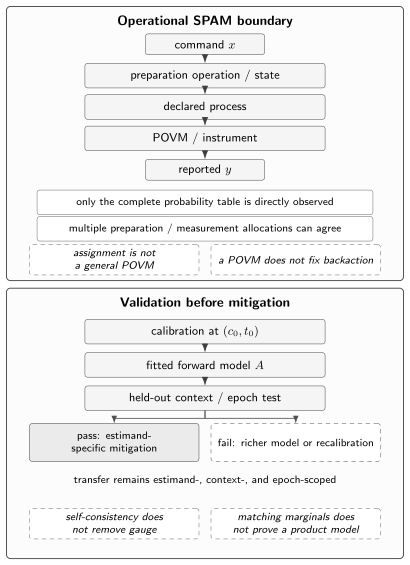
Preparation, process, measurement, identifiability, and held-out SPAM validation boundaries — Observed probabilities compose preparation, process, and measurement. Separating the boundaries needs trusted interventions or a self-consistent model with gauge retained; mitigation is licensed only after held-out context and epoch tests.

Context, Drift, Memory, and Correlated SPAM

Context-indexed preparations and detectors

Preparation and measurement models may depend on spectator state, simultaneous operations, previous reset or readout, integration window, classifier version, and acquisition epoch. For a shared latent variable $\lambda$ whose distribution may depend on command $x$ and context $c$ ,

p(y|x,c) = \mathbb E_{\lambda|x,c} \operatorname{Tr}\!\left(M_{y,\lambda}\rho_{x,\lambda}\right).

When preparation and detector fluctuations share $\lambda$ , this generally differs from

\operatorname{Tr}\!\left[ \mathbb E_{\lambda|x,c}(M_{y,\lambda}) \mathbb E_{\lambda|x,c}(\rho_{x,\lambda}) \right].

Averaging each boundary separately has discarded their covariance. This is a SPAM correlation statement, not yet a claim about which hardware component creates the shared variable.

Drift and randomized acquisition

Drift can imitate state dependence when commands are acquired in blocks and can invalidate a later correction even when the calibration fit was excellent. Proctor et al. (2020) give time-resolved methods for detecting and tracking drift, while van Enk and Blume-Kohout (2013) show how source drift breaks ordinary tomography assumptions. Retain timestamps, randomize or raster command order, interleave references, and define epochs or change points before pooling.

An averaged response transfers to mixed-epoch science data only if calibration and science use the same epoch weights, the latent science distribution $\mathbf p$ is epoch independent, and the linear response is stable within the model. If harder states occur preferentially during a worse detector epoch, replacing the sequence by an average matrix loses the correlation that controls the observed frequency. Randomization can balance weights; it cannot justify pooling after a detected model change.

Detector memory and joint-outcome correlations

For several reported bits, the product law

A_{\mathbf y|\mathbf z,c} = \prod_jA^{(j)}_{y_j|z_j,c}

asserts both conditional independence and response locality: each factor is independent of the other reported bits and of every other latent $z_k$ . Matching one-bit marginals proves neither condition. Bravyi et al. (2021) analyze correlated multiqubit response and mitigation overhead, and Chen et al. (2019) demonstrate the importance of simultaneous readout context. Compare isolated and simultaneous calibrations and reserve complete bit patterns as holdouts.

Correlated outputs alone do not locate the cause in measurement. Intended input correlation, preparation error, gates, leakage, shared electronics, and postprocessing are alternatives. A connected witness needs trusted product preparation or explicit preparation bounds; Jackson and van Enk (2015) provide a model-aware route to testing correlated SPAM. For temporal memory, vary the delay between reads and retain the first result, conditional state, invalid outcomes, and later records. Relaxation, measurement disturbance, classifier history, and genuine QND behavior must not be collapsed into one persistence number.

Characterization, Validation, and Transfer

Calibration is an experiment, not a truth source

A calibration data set is an experiment performed under named settings and at a dated epoch. Separate data used to choose the model, tune thresholds, and fit parameters from data used to validate predictions. Record calibration and science shot counts, acceptance, parameter covariance, shared-calibration covariance, residuals, condition measures, and software or classifier provenance.

Detector calibration based on imperfect preparation estimates $C$ , not $A$ , unless preparation is trusted or bounded. Conversely, calibrating preparation with the same untested detector merely closes the loop. D’Ariano et al. (2004), Lundeen et al. (2009), and Lin et al. (2021) each make the role of additional trusted resources or structural assumptions visible. Calibration becomes evidence for transfer only after the fitted object survives an independent test in the intended domain.

Identifiability, uncertainty, and validity windows

Identifiability asks whether distinct admissible parameters generate the same probability law. Conditioning asks how strongly finite noise is amplified along directions that are, in principle, distinguishable. Model validity asks whether the probability law itself describes the relevant data. These are separate questions: more shots do not cure exact nonidentifiability, a well-conditioned inverse does not validate a response model, and a good fit does not ensure future stationarity.

A result should therefore state identifiable combinations, gauge convention, sampling and calibration uncertainty, model-discrepancy checks, and the contexts and epochs for which it was validated. Mogilevtsev et al. (2013) use cross-validated tomography to expose predictive failure on held-out data. A validity window should have an operational expiry rule—elapsed time, classifier revision, residual alarm, context change, or failed interleaved reference—not merely a date in a notebook.

Falsifiers and scoped absence claims

A stress test is useful when its controlled change targets a model assumption and its rejection threshold is derived before examining the holdout. The following designs distinguish what is changed, what is observed, and what a rejection can license.

Stress test	Controlled change	Recorded output	Null model	Falsifier	Licensed inference	Owner
Preparation intervention	Swap or independently bound a preparation while holding detector setting and schedule fixed	Full outcome table, acceptance, invalid records, and reference result	One detector response explains both preparations under the declared bounds	Difference exceeds propagated preparation bounds and finite-shot threshold	The joint model or assumed preparation bound fails; detector-only attribution still needs alternatives	State Tomography
Measurement intervention	Change basis, detector path, or trusted probe while holding the prepared object fixed	Setting-resolved frequencies and, when available, conditional outputs	One POVM or instrument predicts all settings after declared rotations	Held-out frequencies or repeated outputs violate the fitted model	The restricted measurement model fails in the tested setting domain	Measurement Tomography
Simultaneous or spectator context	Toggle remote state, drive, measurement, or reset while preserving the local command	Context-tagged local and joint outcomes with timestamps	Local response is independent of the remote context	A predeclared context contrast exceeds uncertainty and drift controls	Operational context independence is rejected for named schedules, not universally	Leakage and Crosstalk
Randomized epoch or drift	Interleave commands and references across time or compare declared change points	Time-tagged outcomes, reference traces, and fit residuals	One stationary response and preparation law covers all epochs	Time-resolved residual or change statistic crosses its calibrated threshold	Stationarity is rejected above stated sensitivity and resolution	Device Characterization
Repeated-readout or history	Vary prior outcome, reset, retry count, and delay before the next read	Joint temporal records, accepted branches, and conditional states	Current response depends only on current latent state and setting	Later distributions depend on retained history beyond modeled relaxation	Memoryless response is rejected; mechanism needs further intervention	Control, Readout, and Calibration
Joint-outcome product test	Prepare trusted product probes and vary complete simultaneous bit patterns	Full joint distribution and one-bit marginals	Conditional independence and response locality factorize the response	Held-out joint cells disagree although marginal checks pass	The product response is rejected under the stated preparation bounds	Device Characterization

An absence claim may say only that no violation above a derived sensitivity was detected for the named preparations, detectors, contexts, epochs, and trust bounds. It may not promote finite agreement to proof of independence, stationarity, absence of leakage, or universal calibration transfer.

Mitigation Changes Estimators, Not Devices

Forward models and estimand-specific correction

A validated forward model maps a latent distribution or target expectation to observed records. A correction constructs an estimator of one specified latent quantity from those records. It does not reverse the laboratory evolution. Maciejewski et al. (2020) formulate classical postprocessing from detector models, while Bravyi et al. (2021) show that correlated structure and overhead matter for multiqubit experiments.

Error Mitigation Overview owns cross-family estimator selection, covariance, acceptance, total-resource, stacking, and held-out validation rules once a mitigation license is established; this page retains preparation–measurement boundary objects, assignment licenses, identifiability, context transfer, and measurement-specific failure modes.

The correction license names the estimand, preparation ensemble, outcome alphabet, context, epoch, accepted sectors, and model tests. A response validated for terminal computational-basis populations does not automatically correct arbitrary POVMs, conditional states, mid-circuit feedback, or nonlinear postselection. Measurement Error Mitigation owns the subsequent terminal classical-response inference: detector response versus empirical confusion, rank and conditioning, inverse, constrained, likelihood, unfolding, and observable-dual estimators, structured scaling, science and calibration covariance, and drift-qualified held-out validation. This page retains the assignment license, preparation–measurement nonidentifiability, context transfer, attribution, and the decision to reject or enlarge the response model.

Inversion, regularization, and variance cost

For a known square invertible assignment matrix $A$ and $N$ multinomial science shots,

\widehat{\mathbf p}=A^{-1}\widehat{\mathbf q},

\operatorname{Cov}(\widehat{\mathbf p}\mid A) = A^{-1} \frac{\operatorname{diag}(\mathbf q)-\mathbf q\mathbf q^{\mathsf T}}{N} (A^{-1})^{\mathsf T}.

Calibration uncertainty and covariance shared between calibration and science add further terms; model discrepancy is not a covariance correction. Negative components of an unconstrained inverse estimate are not negative physical probabilities. Clipping or projecting to a simplex changes the estimator and introduces bias. Regularization trades variance and instability for bias and must be evaluated on the downstream estimand.

In the binary case inversion requires exactly $1-\alpha-\beta\ne0$ . A small magnitude amplifies variance. The region $\alpha+\beta>1$ is not singular by itself; it describes anticorrelated labels that may be relabeled. Replacing the condition by $\alpha+\beta<1$ would incorrectly discard an invertible response.

Preparation error is not terminal readout error

Measurement mitigation does not repair preparation, measurement backaction, intervening gates, leakage, loss, or the device. It changes an estimate under a forward model and can add calibration cost, sampling overhead, covariance, rejection, and failure modes. A corrected terminal population can still describe a wrongly prepared state, and a corrected first outcome does not make a destructive instrument QND.

Reference randomized benchmarking provides another useful boundary: under its declared model, fixed leading SPAM enters through nuisance amplitude and offset terms, but the protocol does not estimate SPAM. Magesan, Gambetta, and Emerson (2012) derive the standard benchmarking form; drift, context dependence, leakage, or model failure can escape those nuisance terms. Randomized Benchmarking owns the protocol, and Quantum Measurement as Estimation owns the broader estimator theory.

Three Reproducible Finite Audits

Audit 1 — Computational assignment data do not fix a POVM

Consider $E_0^{\rm diag}=\bigl(\begin{smallmatrix}0.93&0\\0&0.12\end{smallmatrix}\bigr)$ and $E_0^{\rm tilt}=\bigl(\begin{smallmatrix}0.93&0.15\\0.15&0.12\end{smallmatrix}\bigr)$ . Both effects and their complements are positive. Their basis-state probabilities agree, $p(0|0)=0.93$ and $p(0|1)=0.12$ , while the plus-state probabilities are $0.525$ and $0.675$ . The tilted eigenvalues are $0.09311459853336096$ and $0.956885401466639$ .

Outcome effects also fail to fix backaction. Ideal $Z$ Lüders branches $\mathcal L_y(\rho)=\Pi_y\rho\Pi_y$ and measure-and-reprepare branches $\mathcal J_y(\rho)=\operatorname{Tr}(\Pi_y\rho)|+\rangle\langle+|$ have the same POVM. After first outcome zero from $|0\rangle$ , a second $Z$ read gives zero with probabilities one and one half, respectively.

Audit 2 — One confusion table, many SPAM allocations

The finite calculation constructs every $F(e)$ factor and verifies $F(0.10)^2=F(0.18)=F(0)F(0.18)=F(0.05)F(13/90)$ . For true $p_0=0.70$ and $N=10000$ , $e=0.10$ gives $q_0=0.66$ , raw standard deviation $0.004737087712930805$ , and corrected standard deviation $0.005921359641163505$ . At $e=0.49$ , $q_0=0.504$ and the corrected standard deviation is $0.24999199987199566$ .

Those variances condition on exactly known calibration and omit model discrepancy. The near-singular example quantifies conditioning, not nonidentifiability: the factor allocation remains structurally ambiguous even when every matrix is well conditioned.

Audit 3 — Correlation and drift break transfer

Order classical probabilities as $(00,01,10,11)$ and let $X$ be the $2\times2$ classical bit-flip permutation. For $A_{\rm corr}=(1-c)I_4+c(X\otimes X)$ with $c=0.08$ , latent $00$ produces $(0.92,0,0,0.08)$ . The product model with the same one-bit marginals produces $(0.8464,0.0736,0.0736,0.0064)$ . Their total-variation distance is $0.1472$ .

With $E_j=\mathbf 1\{Y_j\ne Z_j\}$ , the error-indicator covariance is $0.0736$ . The parity factor $\mathbb E[(-1)^{E_A+E_B}]$ is $1$ for correlated double flips and $0.7056$ for the product model. This rejects the product response only under trusted product preparation or explicit preparation bounds.

For drift, take $e_0=0.02$ , $e_1=0.18$ , stale average $\bar e=0.10$ , and $p_0=0.75$ acquired entirely at epoch one. The observed $q_0=0.66$ gives stale and contemporaneous estimates $0.70$ and $0.75$ . Average calibration transfers only with matching epoch weights, epoch-independent latent science distribution, and a stable linear response.

const tol = 1e-12;
const fail = (message) => { throw new Error(message); };
const near = (actual, expected, message) => {
  if (Math.abs(actual - expected) > tol) fail(message + `: ${actual}`);
};
const vectorNear = (actual, expected, message) => {
  if (actual.length !== expected.length) fail(message + ': length');
  actual.forEach((value, slot) => near(value, expected[slot], message));
};
const add = (a, b) => a.map((row, r) => row.map((value, col) => value + b[r][col]));
const scale = (factor, a) => a.map((row) => row.map((value) => factor * value));
const multiply = (a, b) => a.map((row) =>
  b[0].map((unused, col) => row.reduce((sum, value, k) => sum + value * b[k][col], 0)));
const apply = (a, v) => a.map((row) => row.reduce((sum, value, k) => sum + value * v[k], 0));
const kron = (a, b) => a.flatMap((rowA) =>
  b.map((rowB) => rowA.flatMap((valueA) => rowB.map((valueB) => valueA * valueB))));
const identity = (n) => Array.from({ length: n }, (unused, r) =>
  Array.from({ length: n }, (unusedAgain, col) => Number(r === col)));
const eigenSymmetric2 = (a) => {
  const middle = (a[0][0] + a[1][1]) / 2;
  const radius = Math.hypot((a[0][0] - a[1][1]) / 2, a[0][1]);
  return [middle - radius, middle + radius];
};
const trace2 = (a) => a[0][0] + a[1][1];
const projectorBranch = (projector, state) => multiply(multiply(projector, state), projector);
const reprepareBranch = (projector, state, output) => scale(trace2(multiply(projector, state)), output);
const effectDiag = [[0.93, 0], [0, 0.12]];
const effectTilt = [[0.93, 0.15], [0.15, 0.12]];
const complement = (effect) => add(identity(2), scale(-1, effect));
[effectDiag, effectTilt, complement(effectDiag), complement(effectTilt)].forEach((effect) => {
  const values = eigenSymmetric2(effect);
  if (values[0] < -tol || values[1] > 1 + tol) fail('invalid effect');
});
vectorNear(eigenSymmetric2(effectTilt),
  [0.09311459853336096, 0.956885401466639], 'tilted spectrum');
near(effectDiag[0][0], 0.93, 'computational zero probability');
near(effectDiag[1][1], 0.12, 'computational one probability');
near(effectDiag[0][0], effectTilt[0][0], 'basis zero');
near(effectDiag[1][1], effectTilt[1][1], 'basis one');
const plus = [Math.SQRT1_2, Math.SQRT1_2];
const expectation = (effect, state) => state.reduce((sum, left, r) =>
  sum + left * effect[r].reduce((inner, value, col) => inner + value * state[col], 0), 0);
near(expectation(effectDiag, plus), 0.525, 'diagonal plus probability');
near(expectation(effectTilt, plus), 0.675, 'tilted plus probability');
const p0 = [[1, 0], [0, 0]];
const p1 = [[0, 0], [0, 1]];
const plusState = [[0.5, 0.5], [0.5, 0.5]];
const zProjectors = [p0, p1];
let firstLTotal = 0;
let firstJTotal = 0;
zProjectors.forEach((projector) => {
  const lProbability = trace2(projectorBranch(projector, plusState));
  const jProbability = trace2(reprepareBranch(projector, plusState, plusState));
  near(lProbability, jProbability, 'same POVM probability');
  firstLTotal += lProbability;
  firstJTotal += jProbability;
});
near(firstLTotal, 1, 'Luders first-outcome normalization');
near(firstJTotal, 1, 'reprepare first-outcome normalization');
const firstL = projectorBranch(p0, p0);
const firstJ = reprepareBranch(p0, p0, plusState);
near(trace2(firstL), trace2(firstJ), 'same first outcome probability');
near(trace2(projectorBranch(p0, firstL)), 1, 'Luders repeat');
near(trace2(projectorBranch(p0, firstJ)), 0.5, 'reprepare repeat');
near(trace2(projectorBranch(p1, firstL)) + trace2(projectorBranch(p0, firstL)), 1, 'Luders normalization');
near(trace2(projectorBranch(p1, firstJ)) + trace2(projectorBranch(p0, firstJ)), 1, 'reprepare normalization');

const flip = (e) => [[1 - e, e], [e, 1 - e]];
const confusion = multiply(flip(0.10), flip(0.10));
vectorNear(confusion.flat(), flip(0.18).flat(), 'equal split');
vectorNear(multiply(flip(0), flip(0.18)).flat(), flip(0.18).flat(), 'readout allocation');
vectorNear(multiply(flip(0.05), flip(13 / 90)).flat(), flip(0.18).flat(), 'unequal split');
const observedZero = (e, truthZero) => e + (1 - 2 * e) * truthZero;
const rawSd = (q, shots) => Math.sqrt(q * (1 - q) / shots);
const correctedSd = (e, q, shots) => rawSd(q, shots) / Math.abs(1 - 2 * e);
near(observedZero(0.10, 0.70), 0.66, 'moderate observed probability');
near(rawSd(0.66, 10000), 0.004737087712930805, 'raw deviation');
near(correctedSd(0.10, 0.66, 10000), 0.005921359641163505, 'corrected deviation');
near(observedZero(0.49, 0.70), 0.504, 'unstable observed probability');
near(correctedSd(0.49, 0.504, 10000), 0.24999199987199566, 'unstable deviation');

const bitFlip = [[0, 1], [1, 0]];
const c = 0.08;
const correlatedResponse = add(scale(1 - c, identity(4)), scale(c, kron(bitFlip, bitFlip)));
const latent00 = [1, 0, 0, 0];
const correlated = apply(correlatedResponse, latent00);
const productResponse = kron(flip(c), flip(c));
const product = apply(productResponse, latent00);
const columnSum = (matrix, col) => matrix.reduce((sum, row) => sum + row[col], 0);
[correlatedResponse, productResponse].forEach((response) => {
  response[0].forEach((unused, col) => near(columnSum(response, col), 1, 'response normalization'));
});
vectorNear(correlated, [0.92, 0, 0, 0.08], 'correlated response');
vectorNear(product, [0.8464, 0.0736, 0.0736, 0.0064], 'product response');
const tv = correlated.reduce((sum, value, slot) => sum + Math.abs(value - product[slot]), 0) / 2;
near(tv, 0.1472, 'total variation');
const bits = [[0, 0], [0, 1], [1, 0], [1, 1]];
const moment = (distribution, fn) => distribution.reduce((sum, probability, slot) =>
  sum + probability * fn(bits[slot]), 0);
const covariance = (distribution) => moment(distribution, ([a, b]) => a * b)
  - moment(distribution, ([a]) => a) * moment(distribution, ([unused, b]) => b);
const parityFactor = (distribution) => moment(distribution, ([a, b]) => ((a + b) % 2 ? -1 : 1));
near(moment(correlated, ([a]) => a), c, 'correlated first marginal');
near(moment(correlated, ([unused, b]) => b), c, 'correlated second marginal');
near(moment(product, ([a]) => a), c, 'product first marginal');
near(moment(product, ([unused, b]) => b), c, 'product second marginal');
near(covariance(correlated), 0.0736, 'error covariance');
near(parityFactor(correlated), 1, 'correlated parity');
near(parityFactor(product), 0.7056, 'product parity');
const e0 = 0.02;
const e1 = 0.18;
const staleAverage = (e0 + e1) / 2;
near(staleAverage, 0.10, 'stale averaged calibration');
const driftObserved = observedZero(e1, 0.75);
const invertZero = (e, q) => (q - e) / (1 - 2 * e);
near(driftObserved, 0.66, 'drift observation');
near(invertZero(staleAverage, driftObserved), 0.70, 'stale correction');
near(invertZero(e1, driftObserved), 0.75, 'current correction');
console.log('SPAM finite audits: PASS');

Canonical Owners and Common Claim Failures

This page owns the operational crosswalk from preparation and measurement boundary objects to identifiability, validation, transfer, and estimator validity. Formal POVM and instrument theory belongs to Quantum Instruments; detector reconstruction to Measurement Tomography; state and process reconstruction to State Tomography and Process Tomography; GST protocols to Device Characterization; hardware acquisition to Control, Readout, and Calibration; and numerical representations to Noise Simulation. The chapter guide routes the broader channel and mitigation sequence.

Treating SPAM as one channel. Preparation, process, and measurement compose in an observed probability, but they do not generally combine into one boundary channel with a unique physical location. Retain the complete probability model and declare any effective relocation.

Calling a confusion table detector-only. $C_{y|x}$ contains actual preparation and measurement. It becomes detector response $A_{y|z}$ only under trusted or bounded preparation and the restricted assignment license.

Equating a POVM with an instrument. Effects predict first outcomes. They do not determine conditional states, backaction, QND behavior, or repeated-readout statistics.

Calling GST SPAM-free or gauge-free without qualification. Self-consistency jointly models the boundaries. It retains gauge and model assumptions; operational gauge-invariant predictions do not certify stationary Markovian dynamics.

Inferring product response from marginals. Tensor-product assignment requires conditional independence and response locality. Matching one-bit errors cannot detect correlated flips, and a joint discrepancy is not detector crosstalk without preparation bounds.

Correcting before validating. Inversion propagates an accepted model; it does not test that model. Report conditioning, calibration uncertainty, model discrepancy checks, holdouts, and the context and epoch validity window before interpreting a corrected estimator.

Exercises

1. Build a preparation replacement map

Let $\rho$ be a normalized density operator on an output space. Prove that $\mathcal R_\rho(X)=\operatorname{Tr}(X)\rho$ is CPTP for an arbitrary finite input space. Then construct a heralded branch that succeeds with probability $s$ and retain its success record.

Solution

Diagonalize $\rho=\sum_a\lambda_a|a\rangle\langle a|$ and choose an input basis $\{|j\rangle\}$ . The Kraus family $K_{aj}=\sqrt{\lambda_a}|a\rangle\langle j|$ gives

\sum_{a,j}K_{aj}XK_{aj}^{\dagger} =\operatorname{Tr}(X)\rho, \qquad \sum_{a,j}K_{aj}^{\dagger}K_{aj}=I_{\rm in}.

Thus the map is CP and TP. For $0\le s\le1$ , take $\mathcal P_{\rm ok}=s\mathcal R_\rho$ and $\mathcal P_{\rm fail}=(1-s)\mathcal R_\tau$ for any density operator $\tau$ on the same output space. Each branch is CP-TNI and their sum is TP. On a normalized reference input, the accepted output is $s\rho$ , its trace is $s$ , and the normalized accepted state is $\rho$ only when $s>0$ . Dropping $s$ would hide throughput and fail the preparation-instrument record.

2. Recover an effective POVM from a confusion matrix

Starting from ideal projectors $\Pi_z$ and a column-stochastic response $A_{y|z}$ , derive the effective effects. State the precise terminal-response license and explain why backaction is not an additional condition on $A$ .

Solution

The law of total probability gives

p(y|\rho)=\sum_zA_{y|z}\operatorname{Tr}(\Pi_z\rho) =\operatorname{Tr}\!\left[\left(\sum_zA_{y|z}\Pi_z\right)\rho\right],

so $M_y^{(A)}=\sum_zA_{y|z}\Pi_z$ . Positivity follows from nonnegative coefficients, and $\sum_yM_y^{(A)}=\sum_z\Pi_z=I$ . The response is licensed at fixed context and fixed alphabet when the actual terminal effects are diagonal in the declared ideal basis and leakage or history has not changed the model. An off-diagonal effect fails this representation even if basis calibration agrees.

The matrix contains only reported conditional probabilities, hence only effective effects. Conditional output states require CP branches $\mathcal I_y$ satisfying $M_y=\mathcal I_y^\dagger(I)$ . Backaction is therefore a separate instrument object, not another property of $A$ . Formal reconstruction should be handed to Measurement Tomography.

3. Separate outcome probabilities from backaction

Construct two binary instruments with the ideal $Z$ POVM that agree on every first outcome but disagree on a repeated $Z$ measurement after outcome zero.

Solution

Let $\Pi_y=|y\rangle\langle y|$ . The Lüders instrument is $\mathcal L_y(\rho)=\Pi_y\rho\Pi_y$ . A measure-and-reprepare instrument is

\mathcal J_y(\rho) = \operatorname{Tr}(\Pi_y\rho)|+\rangle\langle+|.

Both families are CP-TNI and have TP sums. Their effects are $\mathcal L_y^\dagger(I)=\mathcal J_y^\dagger(I)=\Pi_y$ , so the first-outcome law is identical for every input. Starting from $|0\rangle$ and conditioning on first outcome zero, $\mathcal L_0$ leaves $|0\rangle$ , whereas $\mathcal J_0$ emits $|+\rangle$ . A second ideal $Z$ measurement reports zero with probabilities $1$ and $1/2$ . Thus a POVM-level calibration cannot license a repeated-use or QND claim; Quantum Instruments owns the general conditional-map theory.

4. Exhibit a SPAM nonidentifiability family

Derive $C=AB$ , reproduce the symmetric-flip factorization family for $C=F(0.18)$ , and separately verify the similarity gauge of a gate-set sequence.

Solution

If command $x$ produces latent ideal $z$ with probability $B_{z|x}$ and $z$ is reported as $y$ with probability $A_{y|z}$ , then

C_{y|x}=\sum_zA_{y|z}B_{z|x},

which is $C=AB$ . Since $F(a)F(b)=F(a+b-2ab)$ , all of $F(0.10)F(0.10)$ , $F(0)F(0.18)$ , and $F(0.05)F(13/90)$ equal $F(0.18)$ . They assign the same observable confusion to different restricted preparation and readout factors. No shot count chooses among them.

For the gate-set expression, substitute $S|\rho\rangle\!\rangle$ , $SG_gS^{-1}$ , and $\langle\!\langle M|S^{-1}$ . Every adjacent $S^{-1}S$ cancels and the endpoint factors cancel as well, leaving the same sequence probability. This is algebraic invariance for invertible $S$ ; only the part of the orbit whose states, effects, and gates remain admissible has a physical interpretation. Device Characterization owns experimental GST design and model tests.

5. Propagate uncertainty through binary inversion

Derive the asymmetric inversion and conditional multinomial covariance. Add a first-order calibration-uncertainty term and explain what regularization changes.

Solution

From $m_{\rm obs}=(\beta-\alpha)+(1-\alpha-\beta)m$ ,

\widehat m = \frac{\widehat m_{\rm obs}-\widehat\beta+\widehat\alpha} {1-\widehat\alpha-\widehat\beta},

provided the denominator is nonzero. For known square invertible $A$ , linear propagation of multinomial covariance gives

\operatorname{Cov}(\widehat{\mathbf p}|A) =A^{-1}\operatorname{Cov}(\widehat{\mathbf q})(A^{-1})^{\mathsf T}.

If $\theta=(\alpha,\beta)$ is estimated independently with covariance $\Sigma_\theta$ , a first-order additional term for $\widehat m=g(\widehat m_{\rm obs},\widehat\theta)$ is $\nabla_\theta g\,\Sigma_\theta\,\nabla_\theta g^{\mathsf T}$ . Shared data require cross-covariance terms. None of these terms represents model discrepancy. Truncation, ridge inversion, or simplex projection can control variance or inadmissible estimates, but each changes the estimator and introduces bias that must be assessed for the target quantity; Variance and Covariance owns the general propagation rules.

6. Reject product readout and stale calibration

Reproduce the correlated-flip and drift fixtures, identify the preparation assumption behind the correlation witness, and write a properly scoped rejection statement.

Solution

Applying $(1-c)I_4+c(X\otimes X)$ with $c=0.08$ to latent $00$ gives $(0.92,0,0,0.08)$ . The one-bit error is $0.08$ , so the product response gives $(0.92^2,0.92\cdot0.08,0.08\cdot0.92,0.08^2)$ . Half the $\ell_1$ distance is $0.1472$ , the error-indicator covariance is $0.08-0.08^2=0.0736$ , and the parity factors are $1$ and $(1-2\cdot0.08)^2=0.7056$ .

For $e_1=0.18$ and $p_0=0.75$ , $q_0=e_1+(1-2e_1)p_0=0.66$ . Inverting with stale $\bar e=0.10$ gives $0.70$ ; using $e_1$ gives $0.75$ . A defensible conclusion is: “For the named simultaneous context and epoch, the product response and pooled calibration were rejected at the predeclared sensitivity, conditional on trusted product preparation or its stated bounds.” It does not identify detector crosstalk or prove failure in untested contexts.

7. Design a self-consistent held-out SPAM study

Design a study that can test a self-consistent SPAM model without converting fit quality into a universal absence claim.

Solution

Declare the system, sectors, command and outcome alphabets, circuit locations, target gate set, and a model including preparation operations, instruments, leakage outcomes, and named simultaneous contexts. Supply trusted references or quantitative bounds sufficient for the intended attributions. Randomize commands across timestamped acquisition, interleave references, vary spectator and repeated-readout conditions, and retain invalid outcomes and acceptance.

Use one partition to choose the model and thresholds, a second to fit it, and untouched circuits, bit patterns, simultaneous schedules, and later epochs for validation. Report likelihood or residual tests, identifiable combinations, gauge convention, condition measures, sampling and calibration covariance, model alternatives, software and classifier versions, and an expiry rule. Route GST protocol design to Device Characterization and physical acquisition changes to Control, Readout, and Calibration.

A limited conclusion is: “No held-out violation above the derived sensitivity was detected for these preparations, detectors, circuits, contexts, epochs, and trust bounds.” Failure of a holdout licenses rejection or enrichment of the model, not automatic assignment of the discrepancy to preparation or measurement.

References

S. Bravyi, S. Sheldon, A. Kandala, D. C. McKay, and J. M. Gambetta, “Mitigating measurement errors in multiqubit experiments,” Physical Review A 103, 042605 (2021), doi:10.1103/PhysRevA.103.042605.
Y. Chen, M. Farahzad, S. Yoo, and T.-C. Wei, “Detector tomography on IBM quantum computers and mitigation of an imperfect measurement,” Physical Review A 100, 052315 (2019), doi:10.1103/PhysRevA.100.052315.
G. M. D’Ariano, L. Maccone, and P. Lo Presti, “Quantum calibration of measurement instrumentation,” Physical Review Letters 93, 250407 (2004), doi:10.1103/PhysRevLett.93.250407.
O. Di Matteo, J. Gamble, C. Granade, K. Rudinger, and N. Wiebe, “Operational, gauge-free quantum tomography,” Quantum 4, 364 (2020), doi:10.22331/q-2020-11-17-364.
C. Jackson and S. J. van Enk, “Detecting correlated errors in state-preparation-and-measurement tomography,” Physical Review A 92, 042312 (2015), doi:10.1103/PhysRevA.92.042312.
J. Lin, J. J. Wallman, I. Hincks, and R. Laflamme, “Independent state and measurement characterization for quantum computers,” Physical Review Research 3, 033285 (2021), doi:10.1103/PhysRevResearch.3.033285.
J. S. Lundeen, A. Feito, H. Coldenstrodt-Ronge, K. L. Pregnell, Ch. Silberhorn, T. C. Ralph, J. Eisert, M. B. Plenio, and I. A. Walmsley, “Tomography of quantum detectors,” Nature Physics 5, 27–30 (2009), doi:10.1038/nphys1133.
F. B. Maciejewski, Z. Zimborás, and M. Oszmaniec, “Mitigation of readout noise in near-term quantum devices by classical post-processing based on detector tomography,” Quantum 4, 257 (2020), doi:10.22331/q-2020-04-24-257.
E. Magesan, J. M. Gambetta, and J. Emerson, “Characterizing quantum gates via randomized benchmarking,” Physical Review A 85, 042311 (2012), doi:10.1103/PhysRevA.85.042311.
S. T. Merkel, J. M. Gambetta, J. A. Smolin, S. Poletto, A. D. Córcoles, B. R. Johnson, C. A. Ryan, and M. Steffen, “Self-consistent quantum process tomography,” Physical Review A 87, 062119 (2013), doi:10.1103/PhysRevA.87.062119.
D. Mogilevtsev, Z. Hradil, J. Řeháček, and V. S. Shchesnovich, “Cross-validated tomography,” Physical Review Letters 111, 120403 (2013), doi:10.1103/PhysRevLett.111.120403.
E. Nielsen, J. K. Gamble, K. Rudinger, T. Scholten, K. Young, and R. Blume-Kohout, “Gate set tomography,” Quantum 5, 557 (2021), doi:10.22331/q-2021-10-05-557.
T. Proctor, M. Revelle, E. Nielsen, K. Rudinger, D. Lobser, P. Maunz, R. Blume-Kohout, and K. Young, “Detecting and tracking drift in quantum information processors,” Nature Communications 11, 5396 (2020), doi:10.1038/s41467-020-19074-4.
S. J. van Enk and R. Blume-Kohout, “When quantum tomography goes wrong: drift of quantum sources and other errors,” New Journal of Physics 15, 025024 (2013), doi:10.1088/1367-2630/15/2/025024.