Process Tomography

Short Definition

Quantum process tomography reconstructs a linear quantum operation from known input preparations and measured output statistics. For a deterministic channel

$$\mathcal E: \mathcal B(\mathcal H_{\mathrm{in}}) \longrightarrow \mathcal B(\mathcal H_{\mathrm{out}}),$$

ordinary process tomography assumes that $\mathcal E$ is completely positive and trace preserving. An input state $\rho_k$, output setting $s$, and outcome $a$ have modeled probability

$$p(a|k,s,\mathcal E) = \operatorname{Tr} \!\left[ E_{a|s}\,\mathcal E(\rho_k) \right].$$

The input states and output effects must jointly probe every allowed channel direction. Counts then support a linear, constrained, maximum-likelihood, or Bayesian estimate, together with uncertainty and model checks.

Process tomography is not simply State Tomography performed several times. The object has many more parameters, physicality combines complete positivity with trace conditions, errors in both input preparation and output measurement can be assigned incorrectly to the process, and a gate used inside a circuit need not equal the isolated effective channel measured by a tomographic experiment.

This page owns the reconstruction protocols, statistical workflow, SPAM boundary, validation, and scaling. Choi Matrix, Kraus Representation, and Channel–State Duality own the channel representations and their conventions. Metrics for Quantum Hardware owns average gate fidelity, diamond distance, randomized benchmarking, and their operational interpretation. Network Verification owns the distinct decision problem of whether a delivered, possibly heralded network channel and its surrounding service meet a threshold under stated sampling and trust assumptions.

The Statistical Experiment

Suppose input $k$ and measurement setting $s$ are repeated $N_{k,s}$ times, giving counts $n_{a|k,s}$. Under a stationary, independent-shot model,

$$N_{k,s}=\sum_a n_{a|k,s}, \qquad \mathbf n_{k,s} \sim \operatorname{Multinomial} \!\left( N_{k,s},\mathbf p_{k,s} \right).$$

The likelihood, up to count-dependent constants, is

$$\mathcal L(\mathcal E) = \prod_{k,s,a} \left\{ \operatorname{Tr} \!\left[ E_{a|s}\mathcal E(\rho_k) \right] \right\}^{n_{a|k,s}}.$$

This model already declares a trust boundary. The $\rho_k$ are treated as known states, the $E_{a|s}$ as known effects, and every use of the device as one draw from the same map. Violating any of those assumptions changes the estimand.

The process under test also needs a physical boundary. Does it include virtual frame changes, idling before readout, leakage, heralding, reset, neighboring operations, or compiler-generated pulses? A reconstructed matrix is meaningful only after those choices are fixed.

Choi-Space Formulation

Use the unnormalized Choi convention of the canonical Choi Matrix page:

$$J_{\mathcal E} = (\mathcal E\otimes\operatorname{id}) \left( |\Omega\rangle\langle\Omega| \right), \qquad |\Omega\rangle=\sum_i|i\rangle|i\rangle.$$

The first tensor factor is the output and the second is the input reference. The reconstruction rule gives

$$\mathcal E(X) = \operatorname{Tr}_{\mathrm{in}} \!\left[ J_{\mathcal E} \left( I_{\mathrm{out}}\otimes X^{\mathsf T} \right) \right].$$

Consequently each process-tomography probability is linear in the Choi matrix:

$$p(a|k,s,\mathcal E) = \operatorname{Tr} \!\left[ J_{\mathcal E} \left( E_{a|s}\otimes\rho_k^{\mathsf T} \right) \right].$$

This formula is the central design equation. The transpose is basis dependent and must use the same input basis as the Choi convention. Reversing tensor factors without changing the formula produces a silent permutation error.

For a deterministic physical channel,

$$J_{\mathcal E}\succeq0, \qquad \operatorname{Tr}_{\mathrm{out}}J_{\mathcal E} = I_{\mathrm{in}}.$$

Complete positivity is a matrix positivity constraint; trace preservation is a partial-trace constraint. Enforcing only one is not enough.

Identifiability and Parameter Count

Let $d_{\mathrm{in}}$ and $d_{\mathrm{out}}$ be the input and output dimensions. A Hermitian Choi matrix has

$$d_{\mathrm{in}}^2d_{\mathrm{out}}^2$$

real coordinates. Trace preservation imposes $d_{\mathrm{in}}^2$ independent real linear constraints, so the interior dimension of the CPTP channel set is

$$d_{\mathrm{in}}^2 \left( d_{\mathrm{out}}^2-1 \right).$$

For a square $d$-dimensional channel this becomes

$$d^4-d^2.$$

Complete positivity restricts the allowed convex region but does not lower its interior dimension. A low Kraus rank or unitary hypothesis reduces dimension only by adding structure to the model.

Vectorize the Hermitian Choi coordinates into $\mathbf j$. The probabilities have the linear form

$$\mathbf p=\mathbf c+A\mathbf j.$$

The design is informationally complete for the chosen channel model when $A$ has full rank on the model’s tangent space. Standard tomography obtains this by combining:

• input states whose real span is the full Hermitian input-operator space; and
• output effects whose real span is the full Hermitian output-operator space.

As in state tomography, full rank does not guarantee stable inversion. Small singular values amplify shot noise and calibration error. The conditioning of the actual preparation-and-measurement design belongs in the report.

Standard Prepare-and-Measure Tomography

The conventional protocol proceeds in three conceptual steps:

1. prepare an operator-spanning family $\{\rho_k\}$;
2. apply the unknown process to each preparation; and
3. perform informationally complete state tomography on every output.

The phrase “operator-spanning” matters. Density operators lie in an affine trace-one set, but suitable physical states can still span the full Hermitian operator space linearly. For a qubit, a common family is

$$|0\rangle, \quad |1\rangle, \quad |+\rangle, \quad |{+i}\rangle,$$

because their projectors generate

$$\begin{aligned} |0\rangle\langle0|&=\frac12(I+Z), & |1\rangle\langle1|&=\frac12(I-Z), \\ |+\rangle\langle+|&=\frac12(I+X), & |{+i}\rangle\langle{+i}|&=\frac12(I+Y). \end{aligned}$$

The four output states determine the channel’s action on $I$, $X$, $Y$, and $Z$. Reconstructing each output independently and then assembling a channel is transparent, but independent finite-sample estimates need not combine into a completely positive or trace-preserving map. A joint fit to all raw counts can enforce channel constraints and retain cross-setting covariance.

Preparation circuits are part of the measurement apparatus for this purpose. If $|+\rangle$ is made with the same imperfect gate being characterized, the supposed probe is not an independent reference.

Ancilla-Assisted Process Tomography

Ancilla-assisted process tomography prepares one joint state on the input system $S$ and a reference $R$, applies $\mathcal E$ only to $S$, and performs joint state tomography at the output. With

$$|\Phi\rangle = \frac1{\sqrt d} \sum_{i=1}^d|i\rangle_S|i\rangle_R,$$

the output state is the normalized Choi state:

$$\omega_{S'R} = (\mathcal E\otimes\operatorname{id}_R) \left( |\Phi\rangle\langle\Phi| \right) = \frac{J_{\mathcal E}}{d}.$$

Thus one input-state class encodes the whole channel. The resource has not vanished: the output lives on a space of dimension $d^2$, so its unrestricted state tomography still contains order $d^4$ parameters. The protocol also requires a characterized joint input, a stable ancilla, and informationally complete joint measurements.

Maximal entanglement is sufficient and often well conditioned, but entanglement itself is not the mathematical criterion. A bipartite input is tomographically faithful when its operator-Schmidt components span the input operator space. Some separable correlated states can be faithful, while some entangled states are not. Poor operator-Schmidt conditioning amplifies reconstruction error.

Ancilla assistance therefore trades many distinct probe preparations for a larger state-preparation and joint-measurement problem. It moves the trust boundary; it does not remove it.

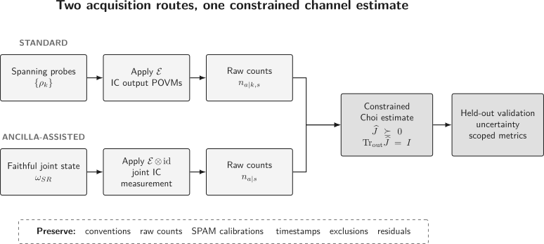
Standard and ancilla-assisted tomography collect different data, but both infer the same declared channel model. In either route, trusted preparations and measurements precede the estimate, while validation and uncertainty follow it.

Representations Are Not Protocols

Quantum Channels for QI owns the convention-complete dictionary among Choi, $\chi$, Pauli-transfer, affine, and Liouville coordinates; this page retains experimental design, estimators, SPAM assumptions, gauge, uncertainty, and holdout validation.

Process matrix in an operator basis

Choose an operator basis $\{A_m\}_{m=0}^{d^2-1}$. A channel can be written

$$\mathcal E(\rho) = \sum_{m,n} \chi_{mn} A_m\rho A_n^\dagger.$$

For a fixed independent basis, complete positivity corresponds to $\chi\succeq0$, while trace preservation requires

$$\sum_{m,n}\chi_{mn}A_n^\dagger A_m=I.$$

The entries of $\chi$ depend on basis ordering and normalization. A bar chart of its real and imaginary parts is not meaningful without those conventions. Diagonalizing $\chi$ can produce a Kraus family, but Kraus operators are not unique and should not be labeled as distinct microscopic error mechanisms without additional evidence.

Transfer matrix

For orthonormal Hermitian bases $\{B_\mu^{\mathrm{out}}\}$ and $\{B_\nu^{\mathrm{in}}\}$, define

$$R_{\mu\nu} = \operatorname{Tr} \!\left[ B_\mu^{\mathrm{out}} \mathcal E(B_\nu^{\mathrm{in}}) \right].$$

This real matrix propagates operator coordinates. In a square basis with $B_0=I/\sqrt d$, trace preservation fixes its first row to

$$R_{0\nu}=\delta_{0\nu}.$$

Unitality constrains the first column instead. Complete positivity is not an elementwise bound on $R$; it is most simply checked after conversion to the Choi matrix.

Choi, process-matrix, transfer-matrix, and Kraus forms describe one fitted map. Changing representation does not create independent evidence or cure a biased experiment.

Reconstruction Methods

Linear inversion

If the design is informationally complete, a pseudoinverse gives an unconstrained estimate

$$\widehat{\mathbf j}_{\mathrm{LI}} = A^+(\mathbf f-\mathbf c).$$

Linear inversion is fast and useful for seeing which data combinations drive which channel elements. Finite counts can yield a Choi matrix with negative eigenvalues or the wrong partial trace. Those violations diagnose sampling fluctuation, ill conditioning, or model mismatch; they do not describe a physical channel.

Constrained least squares

A physical least-squares estimate solves, schematically,

$$\begin{aligned} \widehat J_{\mathrm{CLS}} ={}& \underset{J}{\operatorname{argmin}} \sum_{k,s,a}w_{a|k,s} \left[ f_{a|k,s} - \operatorname{Tr} \!\left( J[E_{a|s}\otimes\rho_k^{\mathsf T}] \right) \right]^2, \\ &J\succeq0, \qquad \operatorname{Tr}_{\mathrm{out}}J=I. \end{aligned}$$

This is convex for fixed nonnegative weights. Projected least squares first computes an unconstrained estimate and then projects it onto the CPTP set. Projection is an estimator choice: the norm, weighting, and projection algorithm affect bias and uncertainty.

Maximum likelihood

The multinomial maximum-likelihood estimator is

$$\widehat J_{\mathrm{ML}} = \underset{J\succeq0,\, \operatorname{Tr}_{\mathrm{out}}J=I} {\operatorname{argmax}} \sum_{k,s,a}n_{a|k,s} \log \operatorname{Tr} \!\left[ J(E_{a|s}\otimes\rho_k^{\mathsf T}) \right].$$

The log-likelihood is concave in $J$ on the convex channel set. Boundary solutions, nonuniqueness under incomplete data, estimator bias, and numerical tolerances still require attention. A physical maximum-likelihood estimate is not proof that the CPTP, stationary, and trusted-SPAM model is adequate.

Structured and regularized estimates

Low Kraus rank, sparsity in a declared process basis, locality, or a near-unitary model can reduce resources. Regularization may use nuclear norms, sparsity penalties, tensor-network structure, or a low-rank factorization. Each gain is conditional on the structural hypothesis and should be tested on held-out data. Selecting the most favorable model after inspecting results without accounting for that selection understates uncertainty.

Worked Example: A Qubit Bit-Flip Channel

Consider

$$\mathcal E_q(\rho) = (1-q)\rho+qX\rho X, \qquad 0\leq q\leq1.$$

In the normalized Pauli basis ordered as $(I,X,Y,Z)$, its transfer matrix is

$$R_q = \operatorname{diag} \left( 1,1,1-2q,1-2q \right).$$

The $X$ component is unchanged, while $Y$ and $Z$ change sign under conjugation by $X$. Preparing $|0\rangle$ and measuring $Z$ gives

$$p(0|0,Z)=1-q.$$

If the observed frequency is $0.92$ under the ideal trusted-SPAM model, then $\widehat q=0.08$. The predictions

$$\begin{aligned} \langle X\rangle_{\mathcal E(|+\rangle)}&=1, \\ \langle Y\rangle_{\mathcal E(|{+i}\rangle)}&=0.84, \\ \langle Z\rangle_{\mathcal E(|0\rangle)}&=0.84 \end{aligned}$$

provide additional tests of the one-parameter model. A discrepancy in the $X$ prediction cannot be repaired by changing $q$; it signals another error or a faulty reference model.

Using $|A\rangle\!\rangle=(A\otimes I)|\Omega\rangle$, the Choi matrix is

$$J_q = (1-q)|I\rangle\!\rangle\langle\!\langle I| + q|X\rangle\!\rangle\langle\!\langle X|.$$

The two vectors are orthogonal and have squared norm $2$. The normalized Choi state $J_q/2$ therefore has eigenvalues $1-q$ and $q$. Relative to the identity channel, the entanglement fidelity is

$$F_e=1-q=0.92,$$

and the average gate fidelity is

$$F_{\mathrm{avg}} = \frac{2F_e+1}{3} \approx 0.9467.$$

These metric conversions are exact only inside the fitted bit-flip CPTP model. Uncertainty in $q$, SPAM, and model mismatch must be propagated to any reported fidelity.

From a Channel Estimate to Metrics

For a $d$-dimensional CPTP map and an ideal unitary $U$, define unnormalized Choi matrices in the same convention. The normalized-Choi overlap is

$$F_e = \frac{1}{d^2} \operatorname{Tr} \!\left( J_{\mathcal E}J_U \right),$$

and

$$F_{\mathrm{avg}} = \frac{dF_e+1}{d+1}.$$

Authors sometimes call $F_e$, its square-root convention, or a normalized $\chi$ overlap “process fidelity.” State the formula rather than relying on the name.

A diamond distance can be computed from a reconstructed channel through semidefinite optimization, but a point estimate of that distance is not a worst-case experimental guarantee. Tomographic uncertainty, SPAM bias, and unseen context dependence remain. Nonlinear metrics should be evaluated over a confidence or credible region when the claim depends on their bounds.

Average fidelity also does not identify error mechanism. Coherent rotation, stochastic Pauli noise, leakage projected back into a computational model, and contextual error can share a similar scalar while accumulating differently in circuits. Noise in Quantum Information develops those distinctions.

The SPAM Identification Problem

Suppose nominal probes are transformed by an unknown preparation map $\mathcal P$, and an output imperfection is represented by a map $\mathcal M$ before an otherwise nominal measurement. The data are

$$p(a|k,s) = \operatorname{Tr} \!\left[ E_{a|s}^{\mathrm{nom}} (\mathcal M\circ\mathcal E\circ\mathcal P) (\rho_k^{\mathrm{nom}}) \right].$$

Standard process tomography that assumes ideal SPAM tends to reconstruct the effective composite

$$\mathcal E_{\mathrm{eff}} = \mathcal M\circ\mathcal E\circ\mathcal P,$$

not $\mathcal E$ alone. More shots reduce counting noise around the wrong answer; they do not identify the factors.

Independent state and measurement calibration can reduce this bias, but those calibrations have their own references and drift. Inverting a noisy calibration map can severely amplify uncertainty and need not be a physical operation.

Gate-set tomography instead fits preparations, measurements, and a library of gates self-consistently from sequences. It has a gauge freedom. In Liouville notation, probabilities are invariant under the schematic transformation

$$|\rho\rangle\!\rangle \mapsto G|\rho\rangle\!\rangle, \quad \langle\!\langle E| \mapsto \langle\!\langle E|G^{-1}, \quad \mathcal G_i \mapsto G\mathcal G_iG^{-1}.$$

Self-consistency moves the problem from trusted SPAM to a relational gate-set model; it does not make every matrix entry absolutely observable. Gauge fixing, model adequacy, sequence context, and uncertainty remain part of the result.

SPAM Errors owns the QI-facing preparation–process–measurement composition, empirical-confusion and assignment distinction, nonidentifiability, gate-set gauge, context transfer, and mitigation license; this page retains channel-reconstruction protocols, Choi-space estimators, uncertainty, validation, and scaling.

When One Channel Is the Wrong Model

Ordinary process tomography assumes that one input-output CPTP map describes each use. That can fail when:

• the initial system and environment are correlated in an input-dependent way;
• the environment retains memory between shots or circuit layers;
• the operation depends on earlier controls, spectator states, or simultaneous gates;
• calibration drifts during the acquisition;
• leakage or loss leaves the declared output space;
• feedback, heralding, or postselection creates outcome-dependent branches.

Aggregating context-dependent maps can produce an effective average, but that average may not predict sequences. A map that fits one-use experiments need not compose as

$$\mathcal E^m$$

for $m$ repeated uses. Sequence residuals and time-blocked tests are therefore essential when the intended claim concerns circuits rather than isolated operations. What Non-Markovian Means gives the broader memory framework. Multi-time process tensors or explicit environment models, rather than a larger one-step Choi matrix, are needed for a general history-dependent experiment.

For a heralded operation, retain the success probability. A trace-nonincreasing map obeys

$$J\succeq0, \qquad \operatorname{Tr}_{\mathrm{out}}J\preceq I.$$

Renormalizing every accepted output estimates the conditional state change but erases the input-dependent success rate. The canonical distinction is developed in Trace-Preserving and Trace-Nonincreasing Maps.

Markovian and Non-Markovian Noise owns the operational decision between one-time channel estimates, interval composition, CP divisibility, and multitime intervention models; this page retains channel-reconstruction protocols, Choi-space estimators, uncertainty, validation, and scaling.

Validation

Hold out experiments

Fit on an operator-spanning subset, then predict outcomes for additional input states, measurement settings, sequence lengths, or contexts. Held-out probes do not need to add new rank; they test whether the fitted channel generalizes.

For counts $n_{a|k,s}$ and predictions $\widehat p_{a|k,s}$, one diagnostic is

$$G^2 = 2\sum_{k,s,a} n_{a|k,s} \log \frac{n_{a|k,s}} {N_{k,s}\widehat p_{a|k,s}},$$

with zero-count terms defined as zero. Calibrated simulations are often needed for a reference distribution because constraints, sparse counts, fitted nuisance parameters, and boundary solutions invalidate a universal naive chi-square rule.

Look for structure in residuals

Residuals should be inspected by input, output basis, time block, qubit subset, neighbor activity, and sequence position. Coherent underrotation may appear as an antisymmetric transfer-matrix pattern; readout mismatch may cluster by outcome; drift may appear as time-correlated residuals. The fitted process matrix alone discards these clues.

Compare representations and estimators correctly

Converting one estimate among Choi, transfer, and $\chi$ representations is an algebra check, not independent validation. Comparing linear inversion, constrained least squares, and maximum likelihood can reveal boundary sensitivity, but all share the same erroneous SPAM model if the references are wrong.

Why Full Process Tomography Does Not Scale

For an $n$-qubit channel, $d=2^n$ and the CPTP interior dimension is

$$16^n-4^n.$$

A dense Choi matrix has dimension $4^n\times4^n$. Conventional local Pauli tomography often uses $4^n$ product input states and $3^n$ product measurement bases, for order

$$12^n$$

preparation-setting configurations before repeated shots, calibration, overcompleteness, or context sweeps. Exact counts depend on design conventions, and one setting supplies several commuting observables, but the exponential barrier is not a bookkeeping artifact.

Ancilla assistance replaces the $4^n$ input family by a characterized joint input, then performs state tomography on $2n$ qubits. Local Pauli measurement bases alone scale as $3^{2n}=9^n$, alongside entangled preparation and ancilla control. It changes the resource profile rather than making unrestricted tomography scalable.

Alternatives answer narrower questions or impose structure:

• randomized benchmarking estimates decay parameters rather than a full channel and has different assumptions;
• direct fidelity estimation targets overlap with an ideal process;
• compressed sensing assumes a sparse or low-rank process in a suitable model;
• local and tensor-network methods assume restricted correlations;
• cycle-level methods characterize compiled layers under selected contexts;
• classical-shadow variants target many observables of a Choi state without uniformly reconstructing it.

No method can estimate an arbitrary $n$-qubit channel to unrestricted accuracy with a resource cost polynomial in $n$. Efficiency comes from changing the question or the model class.

A Defensible Workflow

1. Define the process. State input and output spaces, timing, context, heralding, leakage treatment, and exactly where the operation boundary lies.
2. Fix conventions. Record Choi normalization, tensor order, vectorization, operator-basis order, and endianness.
3. Declare trusted references. Identify preparation circuits, ancillas, measurement effects, calibration epochs, and uncertainty models.
4. Check identifiability and conditioning. Compute design rank and singular values on the CPTP tangent space or chosen structured model.
5. Preserve raw acquisition data. Keep counts, settings, timestamps, exclusions, calibration snapshots, and control artifacts.
6. Fit a declared estimator. Publish likelihood or loss, constraints, regularization, initialization, tolerances, and convergence checks.
7. Quantify uncertainty. Propagate shot, calibration, drift, and selection uncertainty to the reported channel functionals.
8. Validate outside the fit. Use held-out probes, repeated uses, context changes, and residual structure before claiming circuit-level prediction.

What to Report

A mature process-tomography result includes:

• the process boundary and acquisition epoch;
• input/output dimensions, leakage and loss policy, and conditioning events;
• probe states, output POVMs, and how both were calibrated;
• raw and accepted shot counts with exclusions;
• representation conventions and conversion tests;
• estimator objective, physical constraints, regularization, and software;
• uncertainty regions or intervals for the actual reported metrics;
• held-out predictive checks and time/context residuals;
• sensitivity to SPAM and plausible alternative models;
• the distinction between an isolated effective map and an in-circuit claim.

A heat map labeled “experimental process matrix” supplies only a small fraction of this evidence.

Common Mistakes

Confusing a representation with a protocol

Choi, $\chi$, transfer, and Kraus forms are coordinate descriptions. They do not specify which data were collected or which references were trusted.

Forgetting the transpose or tensor order

The Choi probability formula is convention dependent. A hidden swap can still produce a matrix that looks plausible.

Enforcing CP but not trace preservation

A positive Choi matrix may describe a trace-decreasing or trace-increasing map. The partial-trace condition must match the physical process.

Treating CPTP projection as data cleaning

Projection changes the estimator and can bias nonlinear metrics. It cannot make an inadequate model correct.

Assigning SPAM error to the gate

Standard process tomography identifies an effective composite unless preparations and measurements are independently trustworthy.

Interpreting Kraus operators as unique mechanisms

Kraus families have unitary freedom. Microscopic labels require independent physical modeling or interventions.

Assuming one-use agreement predicts circuits

Memory, drift, crosstalk, and coherent accumulation can defeat composition of the fitted map.

Hiding success probability through postselection

Conditional fidelity without accepted throughput can make a lossy operation appear artificially ideal.

Exercises

Exercise 1: Count CPTP channel parameters

Derive the interior dimension of a CPTP map from a $d_{\mathrm{in}}$-dimensional input to a $d_{\mathrm{out}}$-dimensional output.

Solution

The Choi matrix is Hermitian on a space of dimension $d_{\mathrm{in}}d_{\mathrm{out}}$, so it has

$$d_{\mathrm{in}}^2d_{\mathrm{out}}^2$$

real coordinates. Trace preservation requires

$$\operatorname{Tr}_{\mathrm{out}}J=I_{\mathrm{in}},$$

an equality between Hermitian $d_{\mathrm{in}}\times d_{\mathrm{in}}$ matrices and hence $d_{\mathrm{in}}^2$ real linear constraints. At an interior positive-definite Choi matrix, positivity imposes inequalities but no further local dimension reduction. The result is

$$d_{\mathrm{in}}^2 \left(d_{\mathrm{out}}^2-1\right).$$

Exercise 2: Derive the Choi probability formula

Starting from the Choi reconstruction rule, show that

$$\operatorname{Tr} \!\left[E\mathcal E(\rho)\right] = \operatorname{Tr} \!\left[J_{\mathcal E}(E\otimes\rho^{\mathsf T})\right].$$

Solution

Insert

$$\mathcal E(\rho) = \operatorname{Tr}_{\mathrm{in}} \!\left[ J_{\mathcal E} (I_{\mathrm{out}}\otimes\rho^{\mathsf T}) \right].$$

Using the defining property of the partial trace,

$$\operatorname{Tr} \!\left[ E\operatorname{Tr}_{\mathrm{in}}X \right] = \operatorname{Tr} \!\left[ (E\otimes I)X \right],$$

we obtain

$$\operatorname{Tr} \!\left[ (E\otimes I) J_{\mathcal E} (I\otimes\rho^{\mathsf T}) \right].$$

The two tensor-factor operators commute, and cyclicity of the trace yields the desired expression.

Exercise 3: Show that four qubit probes span operator space

Prove that the projectors onto $|0\rangle$, $|1\rangle$, $|+\rangle$, and $|{+i}\rangle$ span all Hermitian qubit operators.

Solution

The first two projectors give

$$I = |0\rangle\langle0|+|1\rangle\langle1|, \qquad Z = |0\rangle\langle0|-|1\rangle\langle1|.$$

The other two give

$$X=2|+\rangle\langle+|-I, \qquad Y=2|{+i}\rangle\langle{+i}|-I.$$

Thus the span contains $I,X,Y,Z$, a basis for Hermitian $2\times2$ operators.

Exercise 4: Test the bit-flip Choi matrix

For

$$J_q = (1-q)|I\rangle\!\rangle\langle\!\langle I| + q|X\rangle\!\rangle\langle\!\langle X|,$$

determine when it is completely positive and show that it is trace preserving for every real $q$ for which the expression is a channel.

Solution

The vectors $|I\rangle\!\rangle$ and $|X\rangle\!\rangle$ are orthogonal with squared norm $2$. The nonzero eigenvalues of $J_q$ are therefore $2(1-q)$ and $2q$. Positivity holds exactly when

$$0\leq q\leq1.$$

For any unitary $U$,

$$\operatorname{Tr}_{\mathrm{out}} |U\rangle\!\rangle\langle\!\langle U| = I.$$

Hence

$$\operatorname{Tr}_{\mathrm{out}}J_q = (1-q)I+qI=I.$$

Outside $0\leq q\leq1$, the linear map remains trace preserving but is not completely positive.

Exercise 5: Recover a channel with an ancilla

For a $d$-dimensional channel, show that applying it to half of $|\Phi\rangle=d^{-1/2}\sum_i|i\rangle|i\rangle$ produces $J_{\mathcal E}/d$. Why does this not reduce the generic parameter count?

Solution

Because

$$|\Phi\rangle\langle\Phi| = \frac1d|\Omega\rangle\langle\Omega|,$$

linearity gives

$$(\mathcal E\otimes\operatorname{id}) (|\Phi\rangle\langle\Phi|) = \frac1d (\mathcal E\otimes\operatorname{id}) (|\Omega\rangle\langle\Omega|) = \frac{J_{\mathcal E}}d.$$

The output is a state on dimension $d^2$. Its density matrix has order $d^4$ entries, with the known marginal imposing the channel constraints. One input preparation therefore packages the information but does not reduce the number of generic channel degrees of freedom.

Exercise 6: Exhibit a SPAM ambiguity

Suppose the intended process is $\mathcal E$, but every nominal input first passes through an unknown invertible channel $\mathcal P$. Show why standard tomography with nominal probes identifies $\mathcal E\circ\mathcal P$ rather than the two factors.

Solution

The observed probabilities are

$$p(a|k,s) = \operatorname{Tr} \!\left[ E_{a|s}\, (\mathcal E\circ\mathcal P)(\rho_k^{\mathrm{nom}}) \right].$$

They have exactly the standard process-tomography form with effective channel $\mathcal E_{\mathrm{eff}}=\mathcal E\circ\mathcal P$. For any alternative factorization

$$\mathcal E\circ\mathcal P = (\mathcal E\circ\mathcal Q^{-1}) \circ (\mathcal Q\circ\mathcal P)$$

that remains inside the allowed model, the same probabilities result. More shots determine the composite more precisely but do not separate preparation from process without an independent reference or additional structure.

Exercise 7: Do not erase heralding probability

A successful branch is

$$\mathcal K(\rho)=\eta U\rho U^\dagger, \qquad 0<\eta<1.$$

Find its Choi partial trace and explain what is lost if every accepted output is renormalized before analysis.

Solution

Its Choi matrix is

$$J_{\mathcal K} = \eta|U\rangle\!\rangle\langle\!\langle U|,$$

so

$$\operatorname{Tr}_{\mathrm{out}}J_{\mathcal K} = \eta I \preceq I.$$

The success probability is

$$\operatorname{Tr}\mathcal K(\rho)=\eta$$

for every normalized input. Conditional on success, the normalized output is $U\rho U^\dagger$, independent of $\eta$. Renormalizing accepted outputs alone therefore makes all $0<\eta\leq1$ look identical and discards throughput, which is part of the physical operation.

Exercise 8: Compare five-qubit scaling counts

For a five-qubit channel, compute the CPTP interior dimension, the conventional $4^n3^n$ preparation-setting count, and the $3^{2n}$ local Pauli basis count for ancilla-assisted output tomography.

Solution

For $n=5$,

$$16^5-4^5 = 1{,}048{,}576-1{,}024 = 1{,}047{,}552.$$

The conventional product design has

$$4^5 3^5 = 12^5 = 248{,}832$$

preparation-setting configurations. Ancilla-assisted tomography measures a ten-qubit state and has

$$3^{10}=59{,}049$$

local Pauli basis settings. These counts omit repeated shots, calibration, overcomplete checks, and the greater difficulty of preparing and measuring the joint system.

Further Connections

• State Tomography for informational completeness, physical estimators, uncertainty, and residual analysis at the state level.
• Shadow Tomography for estimating many selected state observables without claiming a full physical reconstruction; channel-shadow extensions require a separate Choi or input-output contract.
• Randomized Benchmarking for estimating a scalable sequence decay rather than reconstructing the full channel, with a different SPAM contract and different blind spots.
• Choi Matrix for the canonical convention, reconstruction formula, and CP/TP tests.
• Channel–State Duality for normalized Choi states and marginal constraints.
• Measurement Tomography for reconstructing unknown output effects rather than an unknown channel.
• Metrics for Quantum Hardware for average fidelity, diamond distance, leakage, and characterization protocols.
• Device Characterization for combining process estimates with spectroscopy, GST, randomized diagnostics, identifiability analysis, context tests, and held-out prediction.
• Why Benchmarking Is Hard for capability surfaces, context, drift, verification, and evidence scope.

References

1. J. F. Poyatos, J. I. Cirac, and P. Zoller, “Complete characterization of a quantum process: The two-bit quantum gate,” Physical Review Letters 78, 390–393 (1997), doi:10.1103/PhysRevLett.78.390.
2. I. L. Chuang and M. A. Nielsen, “Prescription for experimental determination of the dynamics of a quantum black box,” Journal of Modern Optics 44, 2455–2467 (1997), doi:10.1080/09500349708231894.
3. G. M. D’Ariano and P. Lo Presti, “Quantum tomography for measuring experimentally the matrix elements of an arbitrary quantum operation,” Physical Review Letters 86, 4195–4198 (2001), doi:10.1103/PhysRevLett.86.4195.
4. J. B. Altepeter et al., “Ancilla-assisted quantum process tomography,” Physical Review Letters 90, 193601 (2003), doi:10.1103/PhysRevLett.90.193601.
5. J. Fiurášek and Z. Hradil, “Maximum-likelihood estimation of quantum processes,” Physical Review A 63, 020101(R) (2001), doi:10.1103/PhysRevA.63.020101.
6. M. F. Sacchi, “Maximum-likelihood reconstruction of completely positive maps,” Physical Review A 63, 054104 (2001), doi:10.1103/PhysRevA.63.054104.
7. J. L. O’Brien et al., “Quantum process tomography of a controlled-NOT gate,” Physical Review Letters 93, 080502 (2004), doi:10.1103/PhysRevLett.93.080502.
8. M. Mohseni, A. T. Rezakhani, and D. A. Lidar, “Quantum-process tomography: Resource analysis of different strategies,” Physical Review A 77, 032322 (2008), doi:10.1103/PhysRevA.77.032322.
9. A. Shabani et al., “Efficient measurement of quantum dynamics via compressive sensing,” Physical Review Letters 106, 100401 (2011), doi:10.1103/PhysRevLett.106.100401.
10. M. P. da Silva, O. Landon-Cardinal, and D. Poulin, “Practical characterization of quantum devices without tomography,” Physical Review Letters 107, 210404 (2011), doi:10.1103/PhysRevLett.107.210404.
11. S. T. Merkel et al., “Self-consistent quantum process tomography,” Physical Review A 87, 062119 (2013), doi:10.1103/PhysRevA.87.062119.
12. G. C. Knee, E. Bolduc, J. Leach, and E. M. Gauger, “Quantum process tomography via completely positive and trace-preserving projection,” Physical Review A 98, 062336 (2018), doi:10.1103/PhysRevA.98.062336.
13. E. Nielsen, J. K. Gamble, K. Rudinger, T. Scholten, K. Young, and R. Blume-Kohout, “Gate Set Tomography,” Quantum 5, 557 (2021), doi:10.22331/q-2021-10-05-557.
14. T. Surawy-Stepney, J. Kahn, R. Kueng, and M. Guţă, “Projected least-squares quantum process tomography,” Quantum 6, 844 (2022), doi:10.22331/q-2022-10-20-844.

Summary

• Process tomography infers a declared quantum operation from trusted input states and output measurements.
• The Choi formula makes every observed probability linear in the unknown channel and exposes complete-positivity and trace constraints.
• Standard and ancilla-assisted protocols redistribute preparation and measurement resources but retain the generic order-$d^4$ information burden.
• Linear, constrained, likelihood, and structured estimators have distinct bias, uncertainty, and model assumptions.
• Ordinary tomography generally reconstructs an effective SPAM-composed map; self-consistent gate-set methods move, but do not erase, the trust boundary.
• A one-use CPTP fit does not certify in-circuit behavior under memory, drift, crosstalk, leakage, or postselection.