Cross-Entropy Benchmarking

Short Definition

Cross-entropy benchmarking (XEB) scores samples from an implemented random quantum circuit using probabilities calculated for the corresponding ideal circuit. If the hardware tends to produce bit strings that the ideal circuit assigns unusually high probability, the score is positive. The most common form is linear XEB:

$$\mathcal F_{\mathrm{XEB}}(U;q) = D\sum_x q_U(x)p_U(x)-1, \qquad D=2^n.$$

Here $p_U(x)$ is the ideal output probability of an $n$-qubit circuit $U$, and $q_U(x)$ is the distribution actually sampled by the device. The score can be estimated from measured bit strings without reconstructing $q_U$:

$$\widehat{\mathcal F}_{\mathrm{XEB}} = \frac{1}{M}\sum_{i=1}^{M} \left[D p_U(x_i)-1\right], \qquad x_i\sim q_U.$$

For a sufficiently scrambling circuit, a uniform sampler has expected score zero and ideal sampling has score near one. Under a global depolarizing-mixture model, a circuit-normalized score equals the mixture weight exactly. Outside that model, XEB is a correlation statistic, not automatically a state fidelity, channel fidelity, total-variation guarantee, or certificate of computational advantage.

Canonical Scope

This page owns:

• the random-circuit sampling experiment used by XEB;
• logarithmic cross-entropy difference and linear XEB;
• circuit-specific and Porter–Thomas normalizations;
• shot, circuit, and time-block statistics;
• the assumptions under which XEB tracks a circuit-fidelity parameter;
• classical probability-computation costs, spoofing vulnerabilities, and reporting requirements.

Relative Entropy owns the general information-theoretic definitions. Randomized Benchmarking owns inversion-based group-randomized gate decays, while Cycle Benchmarking owns Pauli-randomized fidelities of fixed scheduled layers. Why Benchmarking Is Hard owns the general benchmark contract. Verification of Quantum Advantage owns the classical resource comparison, hardness argument, anti-spoofing analysis, and independent validation required for the stronger claim; XEB by itself does not supply those ingredients.

The Random-Circuit Sampling Task

Fix an $n$-qubit circuit instance $U$ and the computational-basis input $|0^n\rangle$. Its ideal output state and probabilities are

$$|\psi_U\rangle = U|0^n\rangle, \qquad p_U(x) = |\langle x|\psi_U\rangle|^2, \qquad x\in\{0,1\}^n.$$

The device implements a compiled, noisy version of $U$ and returns bit strings drawn from some distribution $q_U$. Random-circuit sampling asks the device to sample $q_U$ for circuits drawn from a declared ensemble. The ensemble is part of the task. It includes:

• the qubit layout and active subset;
• the initial state and measurement basis;
• the one- and two-qubit gate distributions;
• the entangling-layer pattern and circuit depth;
• compilation, routing, scheduling, and frame conventions;
• the random-seed policy and any circuit rejection rule.

Changing any of these can change scrambling, ideal probability statistics, hardware error, and classical simulation cost. “An XEB score on $n$ qubits” is therefore incomplete without the circuit ensemble and implementation contract.

For each sampled circuit, the experiment has two branches. The quantum branch produces bit strings. The classical branch computes $p_U(x_i)$ for those same strings. XEB combines the two only in post-processing.

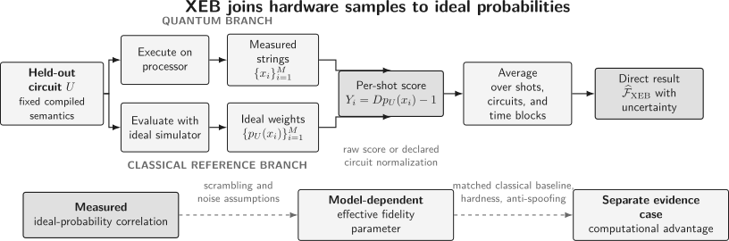
An XEB experiment joins hardware samples with ideal probabilities for the same compiled circuit. The measured score is direct; interpreting it as a fidelity parameter needs a noise-and-scrambling model, and interpreting it as evidence of computational advantage needs a separate classical-hardness analysis.

Cross-Entropy Difference

For distributions $q$ and $p$, their cross-entropy is

$$H(q,p) = - \sum_x q(x)\log p(x).$$

Let $u(x)=1/D$ denote the uniform distribution. The original random-circuit proposal compared the device cross-entropy with the uniform baseline:

$$\begin{aligned} \Delta H(U;q) &= H(u,p_U)-H(q_U,p_U) \\ &= \sum_x \left[q_U(x)-\frac{1}{D}\right] \log p_U(x). \end{aligned}$$

An experimental estimator is

$$\widehat{\Delta H} = H(u,p_U) + \frac{1}{M}\sum_{i=1}^{M}\log p_U(x_i).$$

If $q_U=u$, then $\Delta H=0$. If $q_U=p_U$, the score is

$$\Delta H_{\mathrm{ideal}} = H(u,p_U)-H(p_U).$$

This ideal value depends on the circuit. A circuit-normalized cross-entropy-difference score is therefore

$$\mathcal F_{\log} = \frac{H(u,p_U)-H(q_U,p_U)} {H(u,p_U)-H(p_U)},$$

provided the denominator is nonzero and the required probabilities can be computed reliably.

The logarithm gives very small ideal probabilities large influence. Exact zeros make the score singular, and finite-precision amplitude calculations can produce substantial bias. These numerical and statistical difficulties helped motivate the linear statistic used in most large random-circuit experiments.

Linear XEB Is a Correlation

Define the per-shot weight

$$Y_U(x)=D p_U(x)-1.$$

Linear XEB is its expectation under the device distribution:

$$\mathcal F_{\mathrm{XEB}}(U;q) = \mathbb E_{x\sim q_U}[Y_U(x)].$$

Writing probability vectors in Euclidean coordinates reveals exactly what the score measures:

$$\mathcal F_{\mathrm{XEB}}(U;q) = D\left\langle q_U-u,\, p_U-u \right\rangle.$$

Thus XEB is one projection of the device’s probability error onto the ideal probability fluctuation $p_U-u$. It does not measure every direction in the $D-1$ dimensional probability simplex. If a perturbation $r$ satisfies

$$\sum_x r(x)=0, \qquad \langle r,p_U-u\rangle=0,$$

then $q_U$ and $q_U+r$ have identical linear XEB whenever both are valid distributions. They can nevertheless have different total-variation distance, different marginals, and different higher-order correlations.

The raw score is not confined to $[0,1]$. A distribution concentrated on a largest-probability outcome has

$$\mathcal F_{\mathrm{XEB}} = D p_{\max}-1,$$

which can exceed one. A score may also be negative if samples are anticorrelated with the ideal probabilities. Clipping either case destroys information and invalidates ordinary uncertainty analysis.

Circuit-Specific Normalization

For ideal sampling, the raw score is

$$\mathcal C_U \equiv \mathcal F_{\mathrm{XEB}}(U;p_U) = D\sum_x p_U(x)^2-1.$$

$\mathcal C_U$ is a shifted, rescaled collision probability. It need not equal one, especially for shallow or structured circuits. The circuit-normalized linear XEB estimator is

$$\widehat{\mathcal F}_{\mathrm{uXEB}} = \frac{ D M^{-1}\sum_{i=1}^{M}p_U(x_i)-1 }{ D\sum_x p_U(x)^2-1 }.$$

The label “unbiased” means that its shot expectation is one when samples come from $p_U$, and zero when they come from $u$. It does not mean that every fidelity interpretation is free of model bias.

The normalization fails when $\mathcal C_U=0$. For example, if $p_U$ is exactly uniform, then every sampled bit string has $D p_U(x)-1=0$; no output sampler can be distinguished by this statistic. A very small $\mathcal C_U$ similarly amplifies statistical and numerical error.

Computing $\mathcal C_U$ requires a sum over the full ideal distribution unless an independently justified estimator or ensemble approximation is used. That can be more expensive than calculating probabilities only for observed strings. A report must say whether it used raw XEB, exact circuit-normalized XEB, an ensemble normalization, or a large-$D$ approximation.

Porter–Thomas Statistics

A sufficiently scrambling random circuit is often modeled by a Haar-random state. For a fixed output string, the exact Haar density of $p=|\langle x|\psi\rangle|^2$ is

$$f_D(p) = (D-1)(1-p)^{D-2}, \qquad 0\le p\le1.$$

For large $D$, the scaled probability

$$z=Dp$$

approaches the Porter–Thomas density

$$f(z)=e^{-z}, \qquad z\ge0.$$

The Haar collision moment is

$$\mathbb E_U \left[ \sum_x p_U(x)^2 \right] = \frac{2}{D+1}.$$

Therefore

$$\mathbb E_U[\mathcal C_U] = \frac{D-1}{D+1} \longrightarrow 1.$$

This is why raw linear XEB is commonly described as zero for uniform sampling and one for ideal sampling. The statement is an ensemble, large-$D$ result, not an identity for every finite circuit.

For logarithmic XEB, Porter–Thomas statistics give

$$H(u,p_U) \simeq \log D+\gamma,$$

where $\gamma$ is Euler’s constant, while ideal sampling gives

$$H(p_U) \simeq \log D-1+\gamma.$$

Their difference approaches one. The two notions of XEB therefore share the same convenient Porter–Thomas endpoints but weight probability tails differently.

Anti-concentration and full Porter–Thomas behavior should not be treated as synonyms. The second moment can approach its Haar value before all higher moments and tail properties do. Check the moment relevant to the chosen score and inspect the depth dependence rather than assuming that any random-looking circuit is already in the asymptotic regime.

Exact Meaning Under a Depolarizing Mixture

Consider the output-distribution model

$$q_{U,F}(x) = F p_U(x) + (1-F)\frac{1}{D}, \qquad 0\le F\le1.$$

Substitution gives

$$\mathcal F_{\mathrm{XEB}}(U;q_{U,F}) = F\mathcal C_U.$$

Consequently,

$$\mathcal F_{\mathrm{uXEB}}(U;q_{U,F}) = F.$$

This equality is exact for the stated classical mixture. It is the cleanest interpretation of circuit-normalized XEB.

Suppose instead that the implemented quantum state is modeled as

$$\rho_{U,F} = F|\psi_U\rangle\langle\psi_U| + (1-F)\frac{I}{D}.$$

Its state fidelity with the ideal pure state is

$$\begin{aligned} F_{\mathrm{state}} &= \langle\psi_U|\rho_{U,F}|\psi_U\rangle \\ &= F+\frac{1-F}{D}. \end{aligned}$$

The mixture weight and state fidelity coincide only up to the finite-$D$ offset. More importantly, a general device state need not have this form.

XEB observes only computational-basis probabilities. The fully dephased state

$$\rho_{\mathrm{diag}} = \sum_x p_U(x)|x\rangle\langle x|$$

produces the ideal distribution and hence the ideal XEB score, yet its quantum state fidelity is

$$\langle\psi_U|\rho_{\mathrm{diag}}|\psi_U\rangle = \sum_x p_U(x)^2 \simeq \frac{2}{D}.$$

This is not a defect for the classical sampling task: dephasing immediately before computational-basis measurement does not change that task’s outputs. It does prove that “XEB fidelity” and quantum state fidelity are different concepts unless additional randomized-circuit and noise assumptions connect them.

When XEB Tracks Circuit Fidelity

For sufficiently scrambling circuit ensembles with weak, suitably distributed noise, averaging over circuits can suppress correlations between the ideal probabilities and the error contribution. In that regime, linear XEB, state-preparation fidelity, and a no-error probability may be close. This connection is supported by theory and experiment for specified architectures and noise regimes, but it is not model-free.

The approximation can fail when:

• errors cluster in space or time;
• an error lies near the measurement boundary and affects probabilities differently from state overlap;
• error light cones overlap or cancel;
• the circuit has not scrambled enough;
• nonunital noise, leakage, or loss changes the effective sample space;
• a classical algorithm deliberately creates correlations that score well.

Recent analyses map averaged XEB and fidelity to statistical-mechanical models and find regimes where their agreement breaks down sharply as system size, noise rate, architecture, and entangling power vary. The durable reporting rule is simple: name the theorem, approximation, numerical validation, or empirical control that licenses a fidelity interpretation for the tested regime.

XEB as a Depth-Decay Benchmark

XEB can also be measured over a family of widths and depths. Under a stationary weak-noise model, an ensemble-averaged circuit fidelity may behave as

$$\overline F(m) \simeq A e^{-\lambda m},$$

where $m$ is a declared random-circuit depth, $A$ absorbs approximately depth-independent preparation and measurement effects, and $\lambda$ is an effective error per layer. One may fit

$$\overline{\mathcal F}_{\mathrm{uXEB}}(m) \simeq A e^{-\lambda m}$$

only after verifying that normalized XEB tracks the intended fidelity over the fit window.

An independent component model often predicts

$$F_{\mathrm{prod}} \simeq \prod_{g\in\mathcal G}(1-e_g),$$

or, for small $e_g$,

$$-\log F_{\mathrm{prod}} \simeq \sum_{g\in\mathcal G}e_g.$$

Agreement between an XEB decay and this product can be a useful consistency check. It does not prove that all errors are independent: different correlated models may agree on one scalar. Disagreement is diagnostic but may arise from context-dependent gates, crosstalk, coherent accumulation, leakage, readout, drift, or an invalid XEB-to-fidelity approximation.

Randomized Benchmarking derives group-twirled inversion decays. Cycle Benchmarking derives Pauli-orbit decays for a fixed scheduled layer. Random-circuit XEB instead relies on scrambling and classically evaluated ideal probabilities; it can accommodate non-Clifford circuit ensembles but inherits the classical verification bottleneck.

The Standard Experimental Protocol

A defensible protocol proceeds as follows.

1. Freeze the task. Declare width, depth convention, layout, gate distribution, entangling pattern, compilation policy, measurement map, and allowed post-processing.
2. Separate tuning and evaluation. Generate calibration circuits and held-out evaluation circuits from disjoint recorded seeds.
3. Compile once. Preserve both logical circuits and exact compiled schedules, including inserted gates, routing, frame changes, idles, and disabled qubits.
4. Build the ideal reference. Compute $p_U(x_i)$ for every accepted sample using the exact compiled ideal circuit. Validate the simulator on smaller instances and by independent spot checks.
5. Interleave execution. Mix circuit instances and depths in chronological order so drift is not perfectly confounded with depth or circuit identity.
6. Retain raw outcomes. Store every shot, timestamp, circuit identifier, calibration identifier, and rejection or postselection flag.
7. Score per circuit. Report raw XEB and, when available, circuit-normalized XEB before pooling.
8. Quantify hierarchical uncertainty. Resample or model circuits, shots, and time blocks at the levels at which they were randomized.
9. Fit only declared models. Treat an exponential decay or product formula as a tested model, with residuals and alternatives, not as the definition of XEB.
10. Publish controls and non-claims. Include reduced circuits, simulator checks, drift controls, negative controls, and the claims the score does not support.

Calibration loops can legitimately use XEB as an objective. The reported evaluation score should then come from held-out circuits acquired after the tuning rule was fixed. Calibration Loops develops this training-versus-validation boundary.

Worked Four-Outcome Example

Let

$$p = \left( \frac12,\frac14,\frac18,\frac18 \right), \qquad D=4.$$

The ideal raw score is

$$\begin{aligned} \mathcal C &= 4\left[ \left(\frac12\right)^2 + \left(\frac14\right)^2 + 2\left(\frac18\right)^2 \right]-1 \\ &= \frac38. \end{aligned}$$

This circuit is not Porter–Thomas normalized: ideal sampling scores $3/8$, not one. Now mix ideal and uniform sampling with $F=3/5$:

$$\begin{aligned} q &= \frac35p+\frac25u \\ &= \left( \frac25,\frac14,\frac{7}{40},\frac{7}{40} \right). \end{aligned}$$

The raw score is

$$\mathcal F_{\mathrm{XEB}} = 4\sum_x p(x)q(x)-1 = \frac{9}{40}.$$

Normalizing by $\mathcal C$ gives

$$\mathcal F_{\mathrm{uXEB}} = \frac{9/40}{3/8} = \frac35,$$

which recovers the mixture weight exactly. The total-variation distance is a different quantity:

$$\operatorname{TV}(p,q) = \frac12\sum_x|p(x)-q(x)| = \frac{1}{10}.$$

Nothing in the value $3/5$ alone determines this distance without the mixture model.

Shot Statistics

For a fixed circuit, define

$$Y_i = D p_U(x_i)-1.$$

If shots are independent and identically distributed,

$$\operatorname{SE} \left( \widehat{\mathcal F}_{\mathrm{XEB}} \right) = \sqrt{\frac{\operatorname{Var}_{q_U}(Y)}{M}}.$$

The variance can be estimated from the observed $Y_i$, provided simulator error is negligible and the shots are genuinely independent at the analysis level.

Porter–Thomas statistics give a useful planning approximation. A uniformly selected output has $z=Dp$ distributed approximately as $e^{-z}$. An ideally sampled output has the size-biased density $z e^{-z}$. Under the depolarizing mixture with parameter $F$,

$$\mathbb E[Y]=F$$

and

$$\operatorname{Var}(Y) \simeq 1+2F-F^2.$$

Thus at small $F$,

$$\operatorname{SE} \left( \widehat{\mathcal F}_{\mathrm{XEB}} \right) \simeq \frac{1}{\sqrt M}.$$

Resolving a score of scale $F$ with signal-to-noise ratio $z_\star$ therefore requires roughly

$$M \gtrsim \frac{z_\star^2}{F^2}.$$

This is additive-error efficiency, not constant relative-error efficiency as $F\to0$. A score of order $10^{-3}$ naturally calls for millions of independent samples even before circuit and drift uncertainty are included.

The per-shot statistic has an exponential tail in the Porter–Thomas model. Inspect its empirical distribution, use stable online summation, and report whether uncertainty came from an analytic approximation, nonparametric bootstrap, or likelihood model.

Circuits, Shots, and Time Blocks

Shots from one circuit do not replace independent circuit instances. Let $K$ circuits be evaluated, with $M_k$ shots on circuit $k$. An equal-circuit ensemble estimator is

$$\widehat{\overline F} = \frac{1}{K} \sum_{k=1}^{K}\widehat F_k.$$

A schematic variance decomposition is

$$\operatorname{Var} \left( \widehat{\overline F} \right) \simeq \frac{\sigma_{\mathrm{circ}}^2}{K} + \frac{1}{K^2} \sum_{k=1}^{K} \frac{\sigma_{\mathrm{shot},k}^2}{M_k}.$$

$\sigma_{\mathrm{circ}}^2$ measures true circuit-to-circuit variability; $\sigma_{\mathrm{shot},k}^2$ measures repeated-sampling variability. Deep, strongly scrambling ensembles can have modest circuit variance for some scores, but that is a property to estimate, not a universal permission to use one circuit.

Hardware data add a third level. Shots acquired close in time can share calibration drift, temperature changes, frequency collisions, or queue conditions. If time blocks are the independent experimental units, resampling individual shots produces overconfident intervals. A practical hierarchical bootstrap resamples time blocks, then circuits within each block, then shots within each circuit. Report both between-circuit and between-block spread.

Pooling all shots estimates a shot-weighted circuit ensemble:

$$\widehat F_{\mathrm{pool}} = \frac{\sum_k M_k\widehat F_k}{\sum_k M_k}.$$

It equals the equal-circuit estimator only when shot counts are equal or the weighting is deliberately part of the benchmark. State the target ensemble before choosing the aggregation.

The Classical Reference Bottleneck

Linear XEB does not require reconstructing all of $q_U$, but it does require an ideal probability for each retained output. Exact state-vector simulation computes all amplitudes at exponential memory cost. Schrödinger–Feynman and tensor-network methods can compute selected amplitudes or batches while trading memory for contraction time. Their cost depends strongly on circuit depth, geometry, gate structure, output batching, and approximation tolerance.

Quantum Circuit Simulation owns the simulation-method comparison, and Tensor-Network Simulation owns contraction design and truncation error. For XEB, record:

• simulator name, version, hardware, precision, and contraction strategy;
• whether probabilities are exact, bounded, or approximate;
• how repeated and correlated bit strings are handled;
• independent amplitude or normalization checks;
• wall-clock time, peak memory, energy or hardware allocation when relevant;
• uncertainty propagated from approximate probabilities.

If $\widetilde p_U=p_U+\delta p_U$ is used, the measured statistic targets

$$\widetilde{\mathcal F}_{\mathrm{XEB}} = D\sum_x q_U(x)\widetilde p_U(x)-1,$$

so its reference bias is

$$\Delta_{\mathrm{ref}} = D\sum_x q_U(x)\delta p_U(x).$$

Even zero-mean simulator error under a uniform distribution can be biased when it correlates with the observed samples. A conservative bound is

$$|\Delta_{\mathrm{ref}}| \le D\|\delta p_U\|_\infty.$$

Approximate amplitude methods should provide a sharper, method-specific error analysis whenever possible.

At the scale where ideal probabilities become difficult to compute, direct XEB verification becomes difficult for the same reason. Reduced-width, reduced-depth, patch, or elided circuits can test extrapolation models and implementation consistency. They do not directly measure the target circuit’s score unless a validated argument connects the reduced and target families.

XEB Does Not Determine Distributional Closeness

The total-variation distance between ideal and device outputs is

$$\operatorname{TV}(p_U,q_U) = \frac12\sum_x|p_U(x)-q_U(x)|.$$

Linear XEB supplies one inner product, while total variation depends on all components. No one-to-one conversion exists for arbitrary $q_U$.

An adversarial generator can place probability on a small set of outcomes with large $p_U(x)$ and obtain a high score while remaining far from $p_U$. More generally, a simulator may reproduce the score but miss marginals, correlations, collision probabilities, or other tests. Conversely, a small positive score can be meaningful evidence of correlation in a declared noise model without implying small total variation.

There is a deeper certification limit. For sufficiently flat sampling distributions, device-independent noninteractive certification of small total-variation distance from classical samples can require exponentially many uses of the device. XEB is sample efficient precisely because it asks a narrower, reference-assisted question. Calling it full distribution certification silently changes that question.

Spoofing and the Adversarial Setting

Two settings must be separated.

In the benign setting, the candidate is an honest implementation of the specified quantum circuit, and the task is to estimate an effective physical error under a validated noise model. Circuit-normalized XEB can be a useful and sample-efficient estimator.

In the adversarial setting, any classical algorithm may optimize the reported test. Sampling hardness and XEB-spoofing hardness are different claims. Algorithms can exploit shallow light cones, omit selected entangling gates, factor the circuit into patches, contract favorable tensor-network paths, or target high-probability outputs without accurately sampling the full ideal distribution. Primary results have established both conditional hardness statements and explicit spoofing algorithms in different regimes.

The correct conclusion is not that XEB is useless. It is that an advantage claim requires an evolving classical baseline:

$$\text{advantage evidence} = \text{quantum score and resources} + \text{best classical score and resources} + \text{hardness and anti-spoofing analysis}.$$

The baseline must use the same circuit instances, score definition, acceptance rule, fidelity target, sample count, and resource accounting. A historical runtime estimate is not a permanent lower bound: classical algorithms, contraction orderings, accelerators, and approximation strategies improve.

Composition Exposes a Fidelity Mismatch

Suppose two systems are independent:

$$p(x_1,x_2)=p_1(x_1)p_2(x_2), \qquad q(x_1,x_2)=q_1(x_1)q_2(x_2).$$

Their raw XEB scores obey

$$\mathcal F_{12}+1 = (\mathcal F_1+1)(\mathcal F_2+1).$$

For small positive scores,

$$\mathcal F_{12} \simeq \mathcal F_1+\mathcal F_2,$$

whereas independent state fidelities multiply:

$$F_{\mathrm{state},12} = F_{\mathrm{state},1}F_{\mathrm{state},2}.$$

This different composition law is another proof that raw XEB cannot be identified with fidelity in arbitrary scaling limits. Scrambling and noise conditions are doing real work whenever the two track each other.

Assumptions and Failure Modes

Insufficient scrambling

At shallow depth, $\mathcal C_U$ may differ greatly across circuits and from one. Raw scores then mix device performance with ideal collision structure. Use circuit normalization where feasible and report ideal moments versus depth.

Correlated and coherent errors

Error light cones can overlap, cancel, or remain correlated with ideal probabilities. A one-parameter depolarizing fit can conceal oscillations, context dependence, or multiple decay scales. Compare XEB with independent cycle, leakage, and calibration diagnostics.

State preparation and readout

XEB is not SPAM-free. Preparation and measurement errors alter $q_U$ and usually reduce the score. A depth fit may absorb approximately depth-independent effects into $A$, but drift or depth-dependent readout behavior can bias $\lambda$.

Leakage, loss, and postselection

If some shots leave the computational space or are discarded, define the unconditional outcome alphabet. A conditional score after postselection and the acceptance probability

$$a = \Pr(\text{shot accepted})$$

must both be reported. High conditional XEB at vanishing acceptance is not high unconditional performance.

Drift and non-Markovian noise

Circuits at different depths acquired in separate chronological blocks can turn drift into an apparent decay. Randomize acquisition order, retain timestamps, repeat calibration sentinels, and analyze residuals by time.

Compilation and instance selection

Removing difficult circuits, changing the qubit subset after seeing results, or tuning on evaluation instances changes the benchmark distribution. Freeze selection rules and publish rejected instances with reasons.

Reference-circuit mismatch

Scoring hardware samples against the logical circuit while hardware executed a different routed or synthesized circuit measures the wrong target. The ideal reference must match the declared compiled semantics, including qubit permutations and measurement relabeling.

Finite-precision probabilities

Logarithmic scores are especially sensitive to underflow and tiny probabilities. Linear scores are more stable but can still be biased by correlated approximation error. Record arithmetic precision and perform normalization checks.

Minimum Reporting Record

An XEB result should report at least:

Field	Required content
task	circuit ensemble, width, depths, layout, gate distributions, initial state, and measurement basis
implementation	logical and compiled circuits, compiler version and options, schedules, qubit subset, and calibration identifiers
sampling	circuits per depth, shots per circuit, acquisition order, timestamps, retries, rejection rules, and postselection
score	logarithmic or linear definition, raw or normalized convention, collision normalization, and pooling weights
reference	simulator, version, precision, hardware, algorithm, approximation controls, and probability checks
statistics	shot, circuit, and time-block uncertainty; interval method; multiple-comparison or selection corrections
model	scrambling evidence, noise model, fit window, residuals, and conditions supporting any fidelity interpretation
controls	held-out circuits, reduced or independently simulated instances, drift sentinels, and negative controls
resources	quantum runtime and shots; classical scoring and baseline compute, memory, hardware, and energy policy
claim boundary	what the score establishes and what it does not establish

Machine-readable circuits, seeds, raw bit strings, ideal probabilities, and scoring code are the preferred evidence bundle. Reproducible Notebooks defines the broader artifact contract.

Common Mistakes

Calling every linear score a cross-entropy

Linear XEB replaces the logarithm by $D p-1$. It is related historically and operationally to cross-entropy difference, but it is not itself an entropy.

Assuming ideal score is exactly one

For one finite circuit the ideal raw score is $\mathcal C_U$, not one. State the normalization.

Calling XEB a state fidelity

XEB uses measurement probabilities. A dephased ideal state is a direct counterexample to an unconditional state-fidelity interpretation.

Treating a positive score as distribution certification

One correlation does not determine total-variation distance or all output statistics.

Ignoring the classical scorer

The ideal-probability calculation is part of the experiment. Approximation, precision, and circuit mismatch can bias the result.

Using shots as circuit replicates

Millions of shots on one circuit estimate that circuit precisely, not the declared random-circuit ensemble.

Fitting an exponential by default

An exponential is a noise model. Residual structure, leakage, drift, and insufficient scrambling can invalidate it.

Reporting only accepted samples

Postselection changes the distribution. Report acceptance and unconditional performance.

Equating XEB hardness with sampling hardness

An algorithm can spoof a scalar test without sampling close to the target. The two hardness questions need separate evidence.

Freezing the classical baseline in time

Classical simulation records are empirical and revisable. Comparisons must be dated, reproducible, and rerun against improved methods.

Research Status

The basic XEB estimators, Porter–Thomas limits, and depolarizing-mixture identity are standard. The relation between XEB and physical fidelity outside simple models remains conditional on architecture, scrambling, error strength, and noise structure. Statistical-mechanical analyses have identified noise-driven regimes and transitions in that relation.

The adversarial status is also active. Conditional hardness results coexist with explicit classical spoofing and tensor-network algorithms. Neither side supports the slogan that any nonzero XEB proves advantage or that every XEB experiment is classically trivial. Durable conclusions should name the circuit family, scaling regime, score threshold, classical model, and resource assumptions.

Further Connections

• Why Benchmarking Is Hard supplies the benchmark contract, drift controls, verification boundary, and classical-baseline discipline.
• Metrics for Quantum Hardware compares XEB’s system-level role with component, gate, readout, and volumetric metrics.
• Quantum Volume and Application Benchmarks contrasts XEB with heavy-output generation, derives the quantum-volume threshold, and extends one random-circuit score to volumetric and workload-level evidence.
• Verification of Quantum Advantage places XEB inside the full correctness, hardness, classical-frontier, matched-resource, adversarial, and reproduction evidence chain.
• Randomized Benchmarking derives a different randomized decay whose estimand comes from an inversion experiment rather than ideal output probabilities.
• Cycle Benchmarking estimates dressed scheduled-layer process fidelity through Pauli randomization and orbit decays.
• Process Tomography reconstructs a small channel under trusted-reference assumptions instead of compressing behavior into one random-circuit score.
• Noise in Quantum Information distinguishes stochastic, coherent, correlated, leakage, readout, and drift mechanisms hidden by one scalar.
• Quantum Circuit Simulation and Tensor-Network Simulation develop the classical reference calculations that make XEB possible.
• Claims, Hype, and Evidence Standards separates a benchmark result from a computational-advantage or application claim.

References

1. S. Boixo et al., “Characterizing quantum supremacy in near-term devices,” Nature Physics 14, 595–600 (2018), doi:10.1038/s41567-018-0124-x.
2. C. Neill et al., “A blueprint for demonstrating quantum supremacy with superconducting qubits,” Science 360, 195–199 (2018), doi:10.1126/science.aao4309.
3. A. Bouland, B. Fefferman, C. Nirkhe, and U. Vazirani, “On the complexity and verification of quantum random circuit sampling,” Nature Physics 15, 159–163 (2019), doi:10.1038/s41567-018-0318-2.
4. F. Arute et al., “Quantum supremacy using a programmable superconducting processor,” Nature 574, 505–510 (2019), doi:10.1038/s41586-019-1666-5.
5. D. Hangleiter, M. Kliesch, J. Eisert, and C. Gogolin, “Sample complexity of device-independently certified ‘quantum supremacy’,” Physical Review Letters 122, 210502 (2019), doi:10.1103/PhysRevLett.122.210502.
6. S. Aaronson and S. Gunn, “On the classical hardness of spoofing linear cross-entropy benchmarking,” arXiv:1910.12085 (2019), arXiv:1910.12085.
7. B. Barak, C.-N. Chou, and X. Gao, “Spoofing linear cross-entropy benchmarking in shallow quantum circuits,” in 12th Innovations in Theoretical Computer Science Conference, LIPIcs 185, 30:1–30:20 (2021), doi:10.4230/LIPIcs.ITCS.2021.30.
8. Y. Liu, M. Otten, R. Bassirianjahromi, L. Jiang, and B. Fefferman, “Benchmarking near-term quantum computers via random circuit sampling,” arXiv:2105.05232v2 (2022), arXiv:2105.05232.
9. F. Pan and P. Zhang, “Simulation of quantum circuits using the big-batch tensor network method,” Physical Review Letters 128, 030501 (2022), doi:10.1103/PhysRevLett.128.030501.
10. F. Pan, K. Chen, and P. Zhang, “Solving the sampling problem of the Sycamore quantum circuits,” Physical Review Letters 129, 090502 (2022), doi:10.1103/PhysRevLett.129.090502.
11. G. Kalachev, P. Panteleev, P. Zhou, and M.-H. Yung, “Classical sampling of random quantum circuits with bounded fidelity,” arXiv:2112.15083v3 (2022), arXiv:2112.15083.
12. X. Gao, M. Kalinowski, C.-N. Chou, M. D. Lukin, B. Barak, and S. Choi, “Limitations of linear cross-entropy as a measure for quantum advantage,” PRX Quantum 5, 010334 (2024), doi:10.1103/PRXQuantum.5.010334.
13. B. Ware et al., “A sharp phase transition in linear cross-entropy benchmarking,” arXiv:2305.04954v1 (2023), arXiv:2305.04954.
14. A. Morvan et al., “Phase transitions in random circuit sampling,” Nature 634, 328–333 (2024), doi:10.1038/s41586-024-07998-6.
15. B. Villalonga et al., “A flexible high-performance simulator for verifying and benchmarking quantum circuits implemented on real hardware,” npj Quantum Information 5, 86 (2019), doi:10.1038/s41534-019-0196-1.

Exercises

1. Uniform and ideal endpoints

Show that a uniform sampler has raw linear XEB zero for every normalized ideal distribution. Show that ideal sampling has score $\mathcal C_U$.

Solution

For $u(x)=1/D$,

$$\begin{aligned} \mathcal F_{\mathrm{XEB}}(U;u) &= D\sum_x\frac{1}{D}p_U(x)-1 \\ &= \sum_xp_U(x)-1 =0. \end{aligned}$$

For $q_U=p_U$,

$$\mathcal F_{\mathrm{XEB}}(U;p_U) = D\sum_xp_U(x)^2-1 = \mathcal C_U.$$

Only after a circuit-specific normalization, or in the large-$D$ Porter–Thomas approximation, is the ideal endpoint one.

2. Recover a depolarizing-mixture weight

Let $q_F=Fp+(1-F)u$. Prove that circuit-normalized linear XEB equals $F$. What happens if $p=u$?

Solution

Substitution gives

$$\begin{aligned} D\sum_x q_F(x)p(x)-1 &= FD\sum_xp(x)^2 + (1-F)\sum_xp(x)-1 \\ &= F\left[D\sum_xp(x)^2-1\right] \\ &= F\mathcal C. \end{aligned}$$

Dividing by $\mathcal C$ gives $F$. If $p=u$, then $\mathcal C=0$ and every per-shot weight vanishes. The normalized estimator is undefined because this circuit supplies no XEB contrast.

3. Derive the Porter–Thomas shot variance

In the large-$D$ approximation, let $z=Dp$. Uniformly sampled outputs have density $e^{-z}$ and ideally sampled outputs have density $z e^{-z}$. For $Y=z-1$ and the mixture $q_F=Fp+(1-F)u$, derive $\operatorname{Var}(Y)=1+2F-F^2$.

Solution

For the exponential density,

$$\mathbb E_u[z]=1, \qquad \mathbb E_u[z^2]=2.$$

Hence

$$\mathbb E_u[Y]=0, \qquad \mathbb E_u[Y^2]=1.$$

For the size-biased density $ze^{-z}$,

$$\mathbb E_p[z]=2, \qquad \mathbb E_p[z^2]=6.$$

Therefore

$$\mathbb E_p[Y]=1, \qquad \mathbb E_p[Y^2] = 6-4+1 =3.$$

Under the mixture,

$$\mathbb E[Y]=F, \qquad \mathbb E[Y^2] =(1-F)\cdot1+F\cdot3 =1+2F.$$

Subtracting the squared mean gives

$$\operatorname{Var}(Y) = 1+2F-F^2.$$

4. Estimate a shot budget

Use the small-$F$ Porter–Thomas approximation to estimate the shots needed to resolve $F=2\times10^{-3}$ at a nominal signal-to-noise ratio of five. Why is this not yet a complete experimental budget?

Solution

At small $F$,

$$\operatorname{SE}(\widehat F) \simeq M^{-1/2}.$$

Demanding $F/\operatorname{SE}=5$ gives

$$M \simeq \left(\frac{5}{2\times10^{-3}}\right)^2 = 6.25\times10^6.$$

This counts independent shots under the asymptotic mixture model. A complete budget must also include enough independent circuit instances and time blocks, possible postselection loss, reference-probability error, multiple depths, fit uncertainty, and robustness checks.

5. Construct an XEB-invisible perturbation

For

$$p = \left( \frac12,\frac14,\frac18,\frac18 \right),$$

find a nonzero vector $r$ satisfying $\sum_xr_x=0$ and $r\cdot(p-u)=0$. Explain what it proves.

Solution

The third and fourth ideal probabilities are equal, so choose

$$r = \epsilon(0,0,1,-1).$$

Then

$$\sum_xr_x=0$$

and

$$r\cdot(p-u) = \epsilon \left[ \left(\frac18-\frac14\right) - \left(\frac18-\frac14\right) \right] =0.$$

For sufficiently small $|\epsilon|$, adding $r$ to an interior probability distribution preserves nonnegativity. The modified distribution has the same linear XEB but different probabilities and generally nonzero total-variation distance from the original. One projection cannot reconstruct a distribution.

6. Compare XEB with state fidelity

For an ideal pure state $|\psi\rangle=\sum_x\sqrt{p_x}e^{i\phi_x}|x\rangle$, consider its dephased state

$$\rho_{\mathrm{diag}} = \sum_xp_x|x\rangle\langle x|.$$

Compute its XEB output distribution and state fidelity.

Solution

Computational-basis measurement of $\rho_{\mathrm{diag}}$ gives $q=p$, so its raw XEB is the ideal value

$$\mathcal F_{\mathrm{XEB}} = D\sum_xp_x^2-1.$$

Its state fidelity with $|\psi\rangle$ is

$$\begin{aligned} \langle\psi|\rho_{\mathrm{diag}}|\psi\rangle &= \sum_xp_x|\langle x|\psi\rangle|^2 \\ &= \sum_xp_x^2. \end{aligned}$$

For a Porter–Thomas state this is about $2/D$, even though the output distribution and XEB are ideal. XEB benchmarks the declared measurement sampling task; it is not an unconditional phase-sensitive state test.

7. Derive the product-system law

For independent pairs $(p_1,q_1)$ and $(p_2,q_2)$, prove

$$\mathcal F_{12}+1 = (\mathcal F_1+1)(\mathcal F_2+1).$$

Solution

Let the dimensions be $D_1$ and $D_2$. Independence gives

$$\begin{aligned} \mathcal F_{12}+1 &= D_1D_2 \sum_{x_1,x_2} p_1(x_1)q_1(x_1) p_2(x_2)q_2(x_2) \\ &= \left[ D_1\sum_{x_1}p_1(x_1)q_1(x_1) \right] \left[ D_2\sum_{x_2}p_2(x_2)q_2(x_2) \right] \\ &= (\mathcal F_1+1)(\mathcal F_2+1). \end{aligned}$$

For small scores this is approximately additive, unlike multiplicative independent state fidelity. The mismatch limits any model-free identification of the two quantities.

8. Audit a benchmark claim

An experiment calibrates gates on 50 random circuits, reports the best 10, computes approximate ideal probabilities without error bounds, pools all shots, and states that positive XEB proves quantum advantage. Identify at least five repairs.

Solution

A defensible repair should:

1. separate calibration circuits from held-out evaluation circuits;
2. predeclare the circuit-selection and rejection policy rather than reporting the best instances;
3. publish every evaluation seed and compiled circuit;
4. validate approximate ideal probabilities and propagate reference error;
5. report per-circuit scores and circuit-level uncertainty rather than only a pooled shot interval;
6. block or model chronological drift;
7. state the exact raw or normalized score convention;
8. compare against current classical spoofing and simulation baselines using matched resources and acceptance criteria;
9. avoid equating positive correlation with total-variation certification or computational advantage.

The benchmark can still support a useful hardware-correlation claim after these repairs, but the advantage claim needs the separate hardness and resource case.