Claims, Hype, and Evidence Standards

Quantum information combines mathematics, physics, computer science, engineering, and commercial development. Those communities produce different kinds of evidence. A theorem, a device benchmark, a laboratory demonstration, and a product forecast can all be valuable, but they do not answer the same question.

This page supplies the canonical claim-audit framework for the volume. Its purpose is not automatic skepticism. Its purpose is calibrated belief: state exactly what was shown, under which assumptions, with which comparison, and how far the conclusion travels.

The Claim Is the Unit of Trust

A claim should be small enough to test and specific enough to be wrong. “Quantum computing is faster” is not a testable scientific claim. A usable statement identifies at least:

$$\mathcal C = \bigl( T,\, I,\, O,\, S,\, B,\, R,\, V,\, U,\, \Omega,\, t \bigr),$$

where:

• $T$ is the task;
• $I$ is the input model or promise;
• $O$ is the required output;
• $S$ is the success criterion;
• $B$ is the comparison baseline;
• $R$ is the resource ledger;
• $V$ is the verification procedure;
• $U$ is the uncertainty statement;
• $\Omega$ is the scope of generalization;
• $t$ is the date, software version, calibration epoch, or other time boundary.

This tuple is a checklist, not standard notation. Its value is diagnostic. If one entry is missing, the reader knows exactly what must be supplied before interpreting the headline.

For example, “processor Q solved problem P in ten seconds” remains ambiguous until one knows whether ten seconds includes state preparation, compilation, repeated shots, network latency, decoding, and classical postprocessing; what accuracy was required; which classical algorithm and hardware were used; and how the answer was verified.

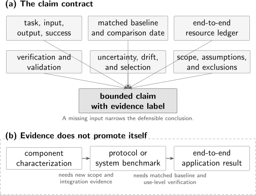
A defensible claim is the intersection of a task contract and an evidence contract. Moving from a component result to a protocol or end-to-end application requires new evidence at each boundary; a stronger adjective cannot perform that promotion.

Claim Labels

Use the narrowest label that the evidence supports.

Label	Required core	What it can establish	What it does not establish by itself
Mathematical theorem	definitions, assumptions, proof	a conclusion follows within a formal model	physical realizability, efficient constants, or experimental performance
Algorithmic speedup under assumptions	problem, access model, algorithm, complexity comparison	asymptotic or finite-cost improvement in a declared model	advantage after data loading, error correction, or hardware overhead
Simulation evidence	model, numerical method, convergence and validation tests	behavior of the simulated model in the checked regime	behavior of an unmodeled device or the asymptotic limit
Experimental demonstration	apparatus, protocol, calibration, data, uncertainty	a component or protocol operated under reported conditions	scalability, fault tolerance, or usefulness
Benchmark result	fixed test, implementation rules, score and uncertainty	performance on that test at that time	universal device quality or application performance
Resource estimate	algorithm, architecture, error model, compiler assumptions	projected resources under a declared scenario	that the assumed hardware or logical rates will be achieved
Engineering projection	milestones, dependencies, risks, schedule model	a technically motivated path	a demonstrated capability or reliable date
Commercial claim	named product, terms, workload and evidence	what an organization asserts or offers	independent scientific validation
Speculative application	mechanism, assumptions, unresolved dependencies	a research direction worth investigating	feasibility, advantage, demand, or deployment

The labels are not a single ladder. A theorem may be deeper than a benchmark while saying less about present hardware. A benchmark may be highly reproducible while saying little about an application. A resource estimate may be internally rigorous while depending on device parameters that do not yet exist.

Compound claims need compound labels

A paper can contain several evidence types:

• a theorem proving hardness under complexity assumptions;
• a numerical estimate for finite instances;
• an experimental sampling result;
• a benchmark against selected classical codes;
• a projection to a future fault-tolerant machine.

These should remain separate sentences. Combining them into “the experiment proved scalable quantum advantage” silently crosses several unsupported boundaries.

The Nine-Question Audit

1. What is the task?

Name the input-output relation. “Optimization,” “simulation,” and “machine learning” are domains, not tasks.

For an optimization problem, specify whether the output must be:

• an exact optimum;
• a feasible point;
• an approximation with a certified ratio;
• a low objective value relative to a reference;
• or samples from a distribution over candidate solutions.

For a sampling task, specify the target distribution and distance criterion. For sensing, specify the parameter, prior or local regime, estimator, and loss function. For communication, specify message type, error, rate, secrecy definition, and adversary.

2. What is the input model?

Input access can determine the apparent speedup. Distinguish:

• an explicit classical list;
• an oracle;
• a succinct circuit;
• a quantum state supplied by another process;
• a stream of experimental data;
• a promise distribution;
• or a family of Hamiltonians with local access.

An algorithm that assumes coherent oracle access to data is not automatically an algorithm for a classical database. The cost of constructing the oracle can dominate the calculation.

3. What output counts as success?

State the tolerance before seeing the answer. Common criteria include

$$\Pr(\text{correct})\geq1-\delta,$$

an additive error

$$\lvert\widehat f-f\rvert\leq\epsilon,$$

or distributional accuracy

$$D(P_{\mathrm{out}},P_{\mathrm{target}}) \leq \epsilon.$$

The distance $D$, confidence level, treatment of failed runs, and aggregation across instances matter. A mean score can conceal a heavy tail or a subgroup on which the method fails.

4. What baseline is used?

A fair comparison holds the task and success criterion fixed. It then reports:

• the classical algorithm and version;
• compiler and numerical-library choices;
• classical hardware and parallelism;
• quantum compiler and calibration;
• preprocessing and postprocessing;
• time limits and stopping rules;
• whether methods were tuned on the test set;
• and the date of the comparison.

“Best known classical” is time-indexed, not permanent. Classical algorithms, tensor-network methods, sampling methods, hardware accelerators, and implementation quality can improve after a quantum result is published.

5. Is the device noisy, error-mitigated, error-detected, or fault-tolerant?

These regimes are distinct.

Regime	What happens to errors?	Appropriate claim
noisy physical execution	errors accumulate in physical operations	device- or circuit-level experimental result
error mitigation	biased estimators are corrected or extrapolated without encoding a protected logical state	mitigated estimate with overhead and assumptions
error detection or postselection	flagged runs are rejected	conditional performance plus acceptance probability
quantum error correction	logical information is encoded and syndromes are used for recovery	logical performance for a specified code and decoder
fault-tolerant operation	errors are controlled throughout preparation, gates, measurement, and recovery	scalable logical claim within a threshold and architecture model

Postselection can increase conditional fidelity while decreasing yield. Report both. Error mitigation can improve an observable estimate while introducing sampling overhead and model dependence. It is not a substitute term for fault tolerance.

6. Is error correction included?

A logical algorithm and a physical implementation are separated by an architecture. A resource estimate should identify:

• code family and distance;
• physical error model and correlations;
• syndrome circuit and decoder;
• logical gate construction;
• magic-state or other non-Clifford resources;
• leakage handling;
• routing and connectivity;
• cycle time and classical feedback latency;
• failure budget assigned to each subroutine.

For a circuit with $N_{\mathrm{loc}}$ relevant failure locations and small logical failure probability $p_L$, a first budgeting estimate is

$$P_{\mathrm{fail}} \lesssim N_{\mathrm{loc}}p_L.$$

This is a union-bound style estimate, not a universal equality. Correlated errors, nonuniform locations, retries, verification, and decoder behavior require a more detailed model.

7. What resources are assumed?

Use a vector, not one headline number:

$$\mathbf R = \bigl( N_{\mathrm{phys}}, N_{\mathrm{log}}, D, N_{\mathrm{shots}}, T, E, M, C_{\mathrm{class}}, P_{\mathrm{succ}} \bigr),$$

where entries may denote physical and logical systems, circuit depth, samples, wall-clock time, energy, memory, classical computation, and success probability.

A useful physical-qubit ledger is

$$N_{\mathrm{phys}} = N_{\mathrm{data}} + N_{\mathrm{syndrome}} + N_{\mathrm{factory}} + N_{\mathrm{routing}} + N_{\mathrm{reserve}}.$$

The terms depend on architecture. Omitting factories, routing, spare capacity, or interconnects can make a precise-looking estimate incomplete.

Likewise, end-to-end time is not only logical depth:

$$T_{\mathrm{end}} = T_{\mathrm{prepare}} + T_{\mathrm{compile}} + T_{\mathrm{execute}} + T_{\mathrm{decode}} + T_{\mathrm{verify}} + T_{\mathrm{classical}}.$$

Some terms can overlap; some can be amortized over many instances. The accounting convention must be explicit.

8. Can the result be verified?

Verification asks whether the claimed output or process is correct relative to a target. The difficulty can grow with system size. If exact classical verification is feasible only for small instances, a large-instance claim needs another strategy:

• hidden tests or held-out circuits;
• interactive verification;
• cross-checks among independent methods;
• conserved quantities or rigorous bounds;
• classically tractable subfamilies;
• extrapolation with a validated error model;
• local observables with known limits;
• cryptographic verification assumptions.

Verification and classical simulation are not identical. Some outputs are hard to generate but easy to check; some sampling distributions are hard both to generate and to verify from finite samples.

9. Does it solve an end-user problem?

A benchmark can be scientifically important without being an application. Ask:

• Is the input representative of a real workload?
• Is the output useful at the achieved accuracy?
• Does the workflow include data acquisition and preparation?
• Is there a competitive non-quantum method?
• Are reliability, latency, energy, throughput, and cost included?
• Does a downstream user receive a better decision or product?

“Application-inspired” and “application-ready” are not synonyms.

Baselines and Speedup Claims

Asymptotic versus finite-instance advantage

Let $C_Q(n,\epsilon)$ and $C_C(n,\epsilon)$ denote quantum and classical costs for problem size $n$ and accuracy $\epsilon$. A speedup ratio is

$$\mathcal S(n,\epsilon) = \frac{C_C(n,\epsilon)} {C_Q(n,\epsilon)}.$$

An asymptotic speedup concerns scaling as $n$ grows. A finite-instance advantage concerns $\mathcal S>1$ over a declared set of instances and hardware. Neither implies the other:

• a better asymptotic scaling can lose at all practical sizes because of constants and overhead;
• a finite benchmark win can disappear when a classical implementation improves;
• a sampling separation can be real while lacking a known end-user application.

State whether the comparison concerns query complexity, gate complexity, sample complexity, memory, wall-clock time, energy, cost, or another resource.

The classical comparator is part of the experiment

The comparator should receive equivalent information and target the same error. A quantum method that estimates an observable to error $\epsilon$ should not be compared with a classical method required to reconstruct an entire state. Conversely, a classical heuristic should not be granted privileged preprocessing that is omitted from its runtime.

Classical Information Review supplies the source, channel, code, decoder, access, error, security, and cost ledger for that baseline; this page owns the evidence label and strength of the resulting claim.

Strong reports include several baselines:

1. a simple reproducible baseline;
2. a competitive tuned baseline;
3. a best-known method from the literature;
4. an ablation showing which quantum component matters.

Negative results are informative. If a classical method wins after careful tuning, that constrains the region in which a quantum advantage claim remains plausible.

Data loading and output extraction

Algorithms stated with state-preparation oracles often exclude data loading. End-to-end claims must restore that cost. Similarly, an exponentially large state space does not produce an exponentially large readable output. If the desired output contains $m$ classical numbers to fixed precision, producing those numbers already incurs output and sampling costs.

Lower Bounds and Limitations owns the formal cross-resource results and their licensed implications; this page retains evidence labels, reporting discipline, uncertainty, matched comparisons, and the language warranted by each level of support.

Uncertainty, Selection, and Reproducibility

Statistical uncertainty

For independent bounded observations $X_i$ with sample mean

$$\overline X = \frac1N \sum_{i=1}^N X_i,$$

the standard error commonly scales as $N^{-1/2}$ under regular conditions. Quantum hardware data can violate simple assumptions through drift, temporal correlations, calibration changes, and adaptive stopping. Report the sampling unit and dependence structure, not only the number of shots.

A complete uncertainty statement distinguishes:

• shot noise;
• calibration uncertainty;
• model mismatch;
• device drift;
• finite-instance variation;
• optimizer randomness;
• classical numerical error;
• and uncertainty in extrapolated hardware parameters.

Postselection and multiple choices

If runs are discarded, report:

$$P_{\mathrm{accept}} = \frac{N_{\mathrm{accepted}}} {N_{\mathrm{attempted}}}$$

alongside conditional accuracy. If many circuits, observables, stopping times, or mitigation settings were tried, state how the reported result was selected. Choosing the best-looking configuration after inspection can bias a benchmark even when every individual measurement is correct.

Reproducibility package

For a durable experimental or benchmark claim, preserve:

• circuit or pulse descriptions;
• raw and processed data;
• calibration records and timestamps;
• software, firmware, compiler, and dependency versions;
• random seeds or instance generators;
• exclusion and postselection rules;
• uncertainty code;
• classical baseline code and hardware details;
• enough metadata to reconstruct figures and tables.

Independent reproduction is stronger than rerunning the same pipeline on the same hidden assumptions. When proprietary constraints prevent full release, list exactly what cannot be audited.

Characterization, Verification, Validation, and Benchmarking

These words are related but not interchangeable.

Activity	Question	Typical output
characterization	What state, process, detector, or noise model describes the component?	estimated parameters or reconstructed model
verification	Is the implementation close enough to a specified target?	acceptance decision, fidelity bound, or witness
validation	Does the model or system predict the relevant real behavior for its intended use?	agreement across held-out observables, regimes, or tasks
benchmarking	How does performance score on a standardized workload or protocol?	metric with implementation rules and uncertainty

No single protocol measures everything. Randomized benchmarking can estimate an averaged gate-performance quantity while reducing sensitivity to state-preparation and measurement errors, but it may not diagnose coherent, correlated, leakage, or context-dependent errors relevant to a specific circuit. Cross-Entropy Benchmarking can detect random-circuit output correlation, but its conversion to fidelity is conditional and the score alone does not certify distributional closeness or computational advantage. Noise in Quantum Information develops these distinctions and the diagnostic hierarchy. Metrics for Quantum Hardware defines the estimands, assumptions, uncertainty, and blind spots of the main characterization protocols. Quantum Volume and Application Benchmarks explains why quantum volume combines several system capabilities in random square circuits but is not an application runtime or a logical-qubit metric.

Application-oriented benchmarks move closer to workloads, yet become more sensitive to compiler choices, instance selection, and classical baselines. A benchmark suite is usually more informative than a universal scalar.

Evidence by Claim Type

Mathematical theorem

Audit definitions, quantifiers, asymptotic regime, oracle model, error tolerance, and complexity assumptions. A conditional hardness result should name the conjecture or hierarchy assumption. “Provable” does not mean assumption-free.

Simulation evidence

Audit discretization, truncation, convergence, finite-size effects, numerical conditioning, stochastic error, and comparison with exact limits. Agreement between two codes is stronger when they use independent algorithms and representations. Error Estimates and Convergence Tests provide the numerical foundation.

Experimental demonstration

Audit controls, calibration, blinding where relevant, drift, uncertainty, excluded data, and alternative explanations. Separate direct observables from model-dependent reconstruction. Data Interpretation and Pitfalls develops this logic for quantum-matter probes.

Benchmark result

Audit the benchmark specification, implementation freedom, pass threshold, statistical rule, instance generator, compiler, and scope. A metric measured after aggressive circuit simplification may be valid, but the simplification policy is part of the benchmark.

Resource estimate

Audit every interface between algorithm, logical circuit, code, architecture, and hardware. Report sensitivity:

$$\frac{\partial\ln R} {\partial\ln \theta_i},$$

or at least rerun the estimate across plausible values of each important assumption $\theta_i$. A range or scenario table is usually more honest than a single integer.

Engineering projection

Audit dependencies and failure modes. A roadmap milestone should identify what observation would falsify the schedule, which advances can proceed in parallel, and which bottleneck controls the critical path.

Commercial claim

Look for a task specification, service-level definition, access conditions, price basis, queueing and latency, data policy, independently reproducible result, and contractually meaningful metric. Press language is not a substitute for methods.

Speculative application

Separate a physical mechanism from a deployable workflow. Label missing algorithms, data interfaces, scaling results, hardware, verification, regulation, or market assumptions. Speculation can be valuable when its dependencies are visible.

Three Worked Claim Audits

Audit 1: a sampling experiment

Claim: “A quantum processor sampled a target circuit distribution faster than a classical computer.”

Required audit:

1. define the circuit ensemble and target distribution;
2. define the distance or score and pass criterion;
3. report device size, depth, fidelity proxy, shots, and postselection;
4. document the classical simulator, approximation error, hardware, and date;
5. explain how large-instance correctness is inferred;
6. distinguish benchmark advantage from useful application value.

The supported label may be experimental benchmark advantage over named classical implementations. A theorem about asymptotic hardness and an experiment at finite noise are separate supporting claims.

Audit 2: below-threshold error correction

Claim: “Logical error decreases as code distance increases.”

Useful evidence compares matched logical experiments at several distances under a stable protocol. A common phenomenological fit is

$$p_L(d,p) \approx A \left( \frac{p}{p_{\mathrm{th}}} \right)^{(d+1)/2},$$

but its meaning depends on code family, decoder, circuit, noise, leakage, and fitted range. Decreasing logical error with distance is evidence for below-threshold behavior in that experiment. It is not by itself a demonstration of an arbitrary fault-tolerant algorithm, a universal threshold, or economical scaling.

Here $A$ is a prefactor, not an additive error floor.

Audit 3: quantum-enhanced sensing

Claim: “The sensor beats the standard quantum limit.”

Define the classical or unentangled comparator and match:

• total probe number;
• interrogation time;
• energy or photon flux;
• bandwidth;
• loss and detector efficiency;
• prior information;
• dead time and duty cycle;
• estimator bias and confidence.

A useful gain is a ratio such as

$$G = \frac{ \mathcal R_{\mathrm{classical}} }{ \mathcal R_{\mathrm{quantum}} },$$

where $\mathcal R$ is the same risk or variance under matched resources. $G>1$ supports an advantage for that task and operating point. It does not establish a universal metrological gain or superior deployed-system cost.

Red Flags

• A headline names no task or error criterion.
• “Exponential” refers only to Hilbert-space dimension.
• The classical comparator is old, untuned, or given a harder output requirement.
• Hardware time excludes compilation, queueing, shots, decoding, or classical optimization.
• Only accepted postselected runs are reported.
• Error bars include shot noise but omit drift or calibration.
• A component fidelity is multiplied into an application claim without validation.
• Physical qubits are described as logical qubits.
• Error mitigation is called fault tolerance.
• A resource estimate reports one number with no parameter sensitivity.
• Verification is performed only where the result is classically easy, then assumed at larger sizes without a validated bridge.
• A benchmark score is treated as universal device rank.
• A commercial roadmap is cited as evidence that a scientific milestone has occurred.
• “Potentially useful” becomes “useful” in a summary.
• A press release broadens the claim beyond the paper’s stated scope.

Reporting Template

A concise defensible statement can use this form:

For task $T$ on input family $I$, system or method $Q$ produced output $O$ with success criterion $S$, using resources $R$. It outperformed or agreed with baseline $B$ under matched conditions. Correctness was assessed by verification $V$, with uncertainty $U$. The result supports claim label $L$ for scope $\Omega$ as of date/version $t$. It does not by itself establish nearest stronger claim.

The last sentence is not self-sabotage. It prevents readers from assigning the result a stronger meaning than the evidence carries.

Exercises

1. Label the evidence

A paper proves that a circuit family is hard to sample classically unless the polynomial hierarchy collapses, numerically simulates 40-qubit instances, and runs 80-qubit instances on hardware. Assign labels to the three results.

Solution

The hardness statement is an algorithmic or complexity-theoretic result under explicit assumptions. The 40-qubit calculations are simulation evidence for finite instances and can support validation of the implementation in that regime. The 80-qubit runs are an experimental demonstration and possibly a benchmark result if a fixed score and comparison protocol are supplied.

None alone proves the others. The theorem may not model finite noise; the simulation may not reach the experimental regime; and the experiment needs a verification bridge before it inherits the theoretical hardness conclusion.

2. Repair a speedup claim

Rewrite “our quantum optimizer is 100 times faster” as a claim contract. List the missing fields rather than inventing values.

Solution

A repaired skeleton is:

For optimization task [missing], on instance distribution [missing] at sizes [missing], the quantum workflow returned outputs meeting [objective/feasibility/approximation criterion] in [time-accounting convention]. This was 100 times lower than [named classical implementation and hardware] under [matched input, accuracy, tuning, and stopping rules]. The quantum cost included [state preparation, circuit execution, shots, optimization, and postprocessing status]. Results were verified by [method] with [uncertainty] as of [software, hardware, and date].

The original sentence omits the task, instances, success criterion, time boundary, baseline, resource ledger, verification, uncertainty, and date.

3. Postselection accounting

Method A has conditional success probability $0.99$ and acceptance probability $0.02$. Method B always returns an answer with success probability $0.90$. If attempts have equal cost and rejected runs are repeated, compare the expected number of correct accepted answers per attempt.

Solution

For A,

$$P(\text{correct accepted}) = 0.02\times0.99 = 0.0198.$$

For B,

$$P(\text{correct output}) =0.90.$$

A has much higher conditional fidelity but far lower throughput per attempt. Which method is preferable depends on whether rejection is allowed, attempt cost, latency, and the consequence of an incorrect answer. Reporting only $0.99$ would hide the dominant resource cost.

4. Logical failure budget

A logical computation contains $10^8$ locations. Using the simple bound

$$P_{\mathrm{fail}} \lesssim N_{\mathrm{loc}}p_L,$$

what logical error per location is required to keep total failure below $1\%$?

Solution

Require

$$10^8p_L \leq 10^{-2},$$

so

$$p_L \leq 10^{-10}.$$

This is a rough budgeting bound. A real estimate should allocate failure across nonuniform operations, state factories, memory, measurement, routing, retries, and correlated faults.

5. Benchmark scope

A processor obtains a high quantum-volume score. State three conclusions that the score can support and three it cannot support by itself.

Solution

It can support:

1. successful execution of the benchmark’s random square circuits up to a reported width and depth;
2. a system-level comparison under the benchmark’s compilation and pass rules;
3. evidence that gate quality, connectivity, and compilation jointly permit that circuit regime.

It cannot by itself establish:

1. performance on a particular chemistry, optimization, or simulation workload;
2. a logical error rate or fault-tolerant capability;
3. universal superiority over another processor or classical computer.

Those conclusions require workload-specific, logical, or comparative evidence.

6. Resource-estimate sensitivity

A projected runtime scales as

$$T \propto \frac{N_Td^2t_c}{P_{\mathrm{factory}}},$$

where $N_T$ is a non-Clifford count, $d$ is code distance, $t_c$ is cycle time, and $P_{\mathrm{factory}}$ is the number of parallel factories. Which parameters deserve the most careful sensitivity analysis?

Solution

The logarithmic sensitivities are

$$\begin{aligned} \frac{\partial\ln T}{\partial\ln N_T}&=1, & \frac{\partial\ln T}{\partial\ln d}&=2, \\ \frac{\partial\ln T}{\partial\ln t_c}&=1, & \frac{\partial\ln T}{\partial\ln P_{\mathrm{factory}}}&=-1. \end{aligned}$$

The quadratic dependence makes uncertainty in $d$ especially influential within this simplified model. However, $d$ is itself chosen from a physical error model and failure budget, while factory parallelism consumes qubits and routing. A credible estimate varies coupled assumptions rather than changing one parameter while holding an inconsistent architecture fixed.

Connections

• What Is Quantum Information? defines the task-and-resource viewpoint used by this audit.
• Quantum Information and Computation maps physical, logical, protocol, and evidence layers.
• Quantum Algorithms and Complexity specializes this page’s evidence discipline to a ten-field algorithm and complexity claim record.
• Quantum Software Stack traces source, target state, dispatched executable, measurement records, postprocessing, and provenance so an implementation claim can be audited at the correct boundary.
• Circuit Intermediate Representations shows which specification, profile, target epoch, output schema, and pass record are needed to audit what an executable actually denotes.
• Resource Estimation Tools supplies the layered contract, uncertainty ledger, validation ladder, and reproducibility bundle required to keep a model-based estimate distinct from a hardware forecast.
• Why Benchmarking Is Hard shows why a score depends on its task ensemble, implementation policy, device epoch, reference, statistics, resources, and scope.
• Reporting Standards supplies the common disclosure record and result-type profiles needed to preserve the evidence behind an audited claim.
• Claims and Evidence Checklist turns this framework into a gate-based review card, comparator test, domain module, and bounded disposition.
• Negative Results and Limitations distinguishes formal barriers, empirical nulls, comparator reversals, resource bottlenecks, and claims that remain open.
• Quantum Illumination applies this audit to a particularly delicate sensing claim by separating an ideal 6 dB error-exponent theorem, structured receivers, matched laboratory advantages, and unestablished field-radar capability.
• Algorithmic Benchmarking states what must be measured before a circuit run becomes evidence about a complete algorithmic task, and why that evidence alone is not an advantage demonstration.
• Verification of Quantum Advantage gives the dedicated audit for correctness, conditional hardness, a dated classical frontier, matched statistical separation, adversarial challenge, and independent reproduction.
• Cross-Entropy Benchmarking shows why a measured random-circuit correlation, a model-dependent fidelity parameter, and computational-advantage evidence are three different claims.
• Evidence Labels supplies site-wide epistemic labels.
• Page Status Labels distinguishes settled, active, conjectural, speculative, and controversial material.
• Data Interpretation and Pitfalls develops cross-probe causal alternatives, mixtures, contacts, surface–bulk distinctions, and history dependence.
• Measurement Tomography covers reconstruction of effective measurement operators from calibration data.
• Living Review Archive separates durable AMO concepts from time-sensitive platform records.

Research Status

The audit principles on this page are durable, but benchmark protocols, classical baselines, hardware records, software stacks, and preferred terminology evolve. Named performance comparisons should be dated and revisited. New evidence should strengthen or narrow a claim by changing an explicit field in the claim contract, not by silently replacing its label.

References

• National Academies of Sciences, Engineering, and Medicine, Quantum Computing: Progress and Prospects, National Academies Press, 2019, doi:10.17226/25196.
• J. Preskill, “Quantum computing in the NISQ era and beyond,” Quantum 2, 79, 2018, doi:10.22331/q-2018-08-06-79.
• J. Eisert, D. Hangleiter, N. Walk, I. Roth, D. Markham, R. Parekh, U. Chabaud, and E. Kashefi, “Quantum certification and benchmarking,” Nature Reviews Physics 2, 382–390, 2020, doi:10.1038/s42254-020-0186-4.
• M. Kliesch and I. Roth, “Theory of quantum system certification,” PRX Quantum 2, 010201, 2021, doi:10.1103/PRXQuantum.2.010201.
• A. Hashim, L. B. Nguyen, N. Goss, B. Marinelli, R. K. Naik, T. Chistolini, J. Hines, et al., “Practical introduction to benchmarking and characterization of quantum computers,” PRX Quantum 6, 030202, 2025, doi:10.1103/PRXQuantum.6.030202.
• A. W. Cross, L. S. Bishop, S. Sheldon, P. D. Nation, and J. M. Gambetta, “Validating quantum computers using randomized model circuits,” Physical Review A 100, 032328, 2019, doi:10.1103/PhysRevA.100.032328.
• T. Proctor, K. Rudinger, K. Young, E. Nielsen, and R. Blume-Kohout, “Measuring the capabilities of quantum computers,” Nature Physics 18, 75–79, 2022, doi:10.1038/s41567-021-01409-7.
• G. D. Kahanamoku-Meyer, S. Choi, U. V. Vazirani, and N. Y. Yao, “Classically verifiable quantum advantage from a computational Bell test,” Nature Physics 18, 918–924, 2022, doi:10.1038/s41567-022-01643-7.
• C. Gidney and M. Ekerå, “How to factor 2048 bit RSA integers in 8 hours using 20 million noisy qubits,” Quantum 5, 433, 2021, doi:10.22331/q-2021-04-15-433.
• E. Knill and R. Laflamme, “Theory of quantum error-correcting codes,” Physical Review A 55, 900–911, 1997, doi:10.1103/PhysRevA.55.900.
• A. Montanaro, “Quantum algorithms: an overview,” npj Quantum Information 2, 15023, 2016, doi:10.1038/npjqi.2015.23.
• K. Bharti, A. Cervera-Lierta, T. H. Kyaw, T. Haug, S. Alperin-Lea, A. Anand, M. Degroote, et al., “Noisy intermediate-scale quantum algorithms,” Reviews of Modern Physics 94, 015004, 2022, doi:10.1103/RevModPhys.94.015004.
• A. Miessen, D. J. Egger, I. Tavernelli, and G. Mazzola, “Benchmarking digital quantum simulations above hundreds of qubits using quantum critical dynamics,” PRX Quantum 5, 040320, 2024, doi:10.1103/PRXQuantum.5.040320.

Summary

Trustworthy quantum-information reporting begins by labeling the evidence correctly. A theorem, simulation, experiment, benchmark, resource estimate, projection, commercial statement, and speculative application carry different warrants. Every consequential claim should expose its task, input, output, success criterion, baseline, resources, verification, uncertainty, scope, and date.

The practical discipline is simple: compare like with like, count the full workflow, report rejected runs and uncertainty, preserve reproducibility metadata, and state the nearest stronger conclusion that has not yet been established.