Standard Quantum Limit

Definition and Scope

In quantum metrology, the standard quantum limit (SQL) usually names the inverse-square-root precision scaling achieved by independent probes under a fixed single-probe resource constraint. If each experimental round uses $N$ probes and the round is repeated independently $\nu$ times, then

$$\Delta\theta_{\mathrm{SQL}} \propto \frac{1}{\sqrt{\nu N}}.$$

The proportionality constant contains the physics of the probe, parameter encoding, interrogation time, contrast, measurement, and units. In a normalized qubit phase-estimation model with an optimal product input and measurement,

$$\Delta\theta_{\mathrm{SQL}} \ge \frac{1}{\sqrt{\nu N}}.$$

This page is the canonical home for the independent-probe SQL, its statistical and Fisher-information derivations, projection-noise and shot-noise examples, resource accounting, and the evidence needed to claim sub-SQL performance. Quantum Measurement as Estimation owns the broader contract connecting a parameterized experiment to a likelihood, estimator, uncertainty statement, and validated claim. Classical and Quantum Fisher Information owns measurement optimization, SLD formulas, and the quantum information metric. Interferometers owns detailed optical implementations. Precision Measurement and Metrology owns clocks and AMO sensor physics. Fisher Information owns the underlying classical statistical quantity.

The name is overloaded. In continuous position measurement, “the SQL” often means an optimum between measurement imprecision and quantum backaction. In laser theory, it can label a model-dependent linewidth. Those are not the same bound as independent-probe scaling. A trustworthy statement names the task and writes the bound rather than relying on the acronym.

Where the 1/√N Law Comes From

Averaging independent outcomes

Suppose one probe produces an outcome $X$ with parameter-dependent mean and variance

$$\mu(\theta) = \mathbb E_\theta[X], \qquad \sigma^2(\theta) = \operatorname{Var}_\theta(X).$$

For $R=\nu N$ independent, identically distributed probe outcomes, the sample mean

$$\overline X_R = \frac{1}{R} \sum_{j=1}^{R}X_j$$

has variance

$$\operatorname{Var}_\theta(\overline X_R) = \frac{\sigma^2(\theta)}{R}.$$

Near an operating point where $\partial_\theta\mu\ne0$, local error propagation gives

$$\Delta\theta \simeq \frac{ \sigma(\theta) }{ \sqrt{\nu N}\, \left| \partial_\theta\mu(\theta) \right| }.$$

The quantum content is in the one-probe distribution: even after technical and detector noise are removed, a probe not prepared in an eigenstate of the readout generally has irreducible outcome variance. Independence then turns that single-probe variance into inverse-square-root scaling.

This argument is local and asymptotic. It assumes a calibrated response, a stable operating point, finite variance, and enough data that the estimator behaves approximately linearly. It does not address phase wrapping, bias, prior information, correlated noise, or an unknown drift shared by every probe.

Fisher-information derivation

Let one measured probe have outcome distribution $p(x\mid\theta)$ and classical Fisher information

$$F_C^{(1)}(\theta) = \sum_x \frac{ \left[ \partial_\theta p(x\mid\theta) \right]^2 }{ p(x\mid\theta) }.$$

Independent likelihoods multiply, log likelihoods add, and Fisher information is additive:

$$F_C^{(R)} = R F_C^{(1)} = \nu N F_C^{(1)}.$$

For a locally unbiased estimator, the classical Cramér–Rao bound therefore gives

$$\operatorname{Var}(\widehat\theta) \ge \frac{1}{ \nu N F_C^{(1)} }.$$

The quantum Fisher information $F_Q$ is the maximum of $F_C$ over allowed measurements. Thus

$$F_C^{(1)} \le F_Q^{(1)},$$

and the independent-probe quantum bound is

$$\Delta\theta \ge \frac{1}{ \sqrt{ \nu N F_Q^{(1)} } }.$$

This is the general SQL formula. The familiar unit-prefactor expression follows only when the parameter and generator are normalized so that the best single probe has $F_Q^{(1)}=1$.

Product and Separable Probe Bound

Consider a unitary encoding on $N$ distinguishable probes,

$$U_\theta = \exp(-i\theta H), \qquad H = \sum_{j=1}^{N}h_j.$$

For a pure state, quantum Fisher information is four times the generator variance:

$$F_Q[|\psi\rangle,H] = 4(\Delta H)^2_\psi.$$

For a product input,

$$\rho_{\mathrm{prod}} = \bigotimes_{j=1}^{N}\rho_j,$$

QFI is additive:

$$F_Q[ \rho_{\mathrm{prod}},H ] = \sum_{j=1}^{N} F_Q[\rho_j,h_j].$$

Let the spectral width of each local generator be bounded by

$$g = \lambda_{\max}(h_j) - \lambda_{\min}(h_j).$$

The maximum one-probe QFI is then $g^2$. Convexity of QFI extends the linear bound to parameter-independent mixtures of product states,

$$\rho_{\mathrm{sep}} = \sum_k p_k \bigotimes_{j=1}^{N} \rho_j^{(k)}:$$ $$F_Q[ \rho_{\mathrm{sep}},H ] \le Ng^2.$$

Consequently,

$$\Delta\theta_{\mathrm{sep}} \ge \frac{1}{ g\sqrt{\nu N} }.$$

For qubits with $h_j=\sigma_z^{(j)}/2$, the spectral width is $g=1$, giving the normalized SQL.

The local resource bound is essential. A bosonic probe with unbounded energy can have unbounded generator variance, so “one probe” is not a complete resource statement. For light, one usually constrains mean photon number, total photon-number sectors, energy through the sample, or channel uses. For spectroscopy, interrogation time belongs in the generator.

Why generator variance can mislead

For pure states under unitary encoding, $F_Q=4(\Delta H)^2$. For mixed states, only

$$F_Q[\rho,H] \le 4(\Delta H)^2_\rho$$

is guaranteed. The variance can contain classical uncertainty that carries no phase information.

For example, consider the incoherent mixture

$$\rho_{\mathrm{mix}} = \frac12 |0\rangle\langle0|^{\otimes N} + \frac12 |1\rangle\langle1|^{\otimes N}$$

with $H=J_z$. Its variance scales as $N^2$, but

$$[\rho_{\mathrm{mix}},J_z]=0,$$

so the state does not change under $\exp(-i\theta J_z)$ and

$$F_Q[\rho_{\mathrm{mix}},J_z] = 0.$$

A large collective variance is therefore not by itself evidence of sub-SQL sensitivity.

Binomial Phase Example

Take one two-outcome probe with

$$\begin{aligned} p_+(\theta) &= \frac{ 1+\sin\theta }{2}, \\ p_-(\theta) &= \frac{ 1-\sin\theta }{2}. \end{aligned}$$

The one-probe Fisher information is

$$\begin{aligned} F_C^{(1)} &= \sum_{s=\pm} \frac{ \left( \partial_\theta p_s \right)^2 }{ p_s } \\ &= 1, \end{aligned}$$

away from support-changing endpoints, where the same value is obtained by a limit.

For $R$ independent probes, the number $K$ of plus outcomes is binomial:

$$K \sim \operatorname{Binomial} \left( R, \frac{1+\sin\theta}{2} \right).$$

At the mid-fringe point $\theta=0$,

$$\mathbb E[K] = \frac{R}{2}, \qquad \operatorname{Var}(K) = \frac{R}{4}.$$

The local estimator

$$\widehat\theta \simeq \frac{2K}{R}-1$$

therefore has

$$\Delta\widehat\theta = \frac{1}{\sqrt R} = \frac{1}{\sqrt{\nu N}}.$$

The same likelihood is realized by ideal Ramsey or two-path interference experiments after a convention-dependent choice of phase origin. The SQL is not tied to one apparatus; it is the information scaling of the independent binary trials.

Projection Noise of Independent Spins

For $N$ two-level probes, define collective spin

$$\mathbf J = \frac12 \sum_{j=1}^{N} \boldsymbol{\sigma}^{(j)}.$$

Prepare each spin along $+x$. The product state has

$$\langle J_x\rangle = \frac N2, \qquad (\Delta J_y)^2 = (\Delta J_z)^2 = \frac N4.$$

Let the parameter generate a rotation about $z$:

$$U_\theta = \exp(-i\theta J_z).$$

Near $\theta=0$,

$$\left. \frac{\partial}{\partial\theta} \langle J_y\rangle_\theta \right|_{\theta=0} = \langle J_x\rangle = \frac N2.$$

Error propagation for one round gives

$$\Delta\theta = \frac{ \Delta J_y }{ \left| \partial_\theta\langle J_y\rangle \right| } = \frac{ \sqrt N/2 }{ N/2 } = \frac{1}{\sqrt N}.$$

After $\nu$ independent rounds,

$$\Delta\theta = \frac{1}{\sqrt{\nu N}}.$$

This is quantum projection noise: each spin measurement gives a discrete outcome even when state preparation and readout are ideal. Detector noise is additional and must be calibrated separately. Ramsey Interferometry develops the pulse sequence and physical spectroscopy.

Optical Shot Noise

An ideal coherent optical mode has Poisson photon-number statistics,

$$\operatorname{Var}(n) = \langle n\rangle = \overline n.$$

In a specified ideal two-path phase measurement, the complete output-count likelihood has Fisher information proportional to the detected mean photon number:

$$F_C = \overline n.$$

The phase uncertainty therefore scales as

$$\Delta\phi_{\mathrm{shot}} \ge \frac{1}{\sqrt{\overline n}}.$$

For $\nu$ identical independent intervals,

$$\Delta\phi_{\mathrm{shot}} \ge \frac{1}{ \sqrt{ \nu\overline n } }.$$

This is the optical shot-noise limit for the declared coherent-state model. It depends on what optical modes and phase references are counted, whether $\overline n$ is incident or detected, and whether loss is assigned to the state, channel, or detector. The full interferometer likelihood and dark-fringe subtleties belong to Interferometers.

Shot Noise, Projection Noise, and the SQL

The terms overlap but are not synonyms in every context.

Term	Typical random variable	Independent-probe behavior	Essential declaration
projection noise	outcomes of uncorrelated atoms, spins, or qubits	variance of a collective count is proportional to $N$	state, basis, contrast, and readout model
optical shot noise	coherent-state photoelectrons or photon counts	Poisson variance equals the mean count	incident or detected flux, modes, bandwidth, and efficiency
standard quantum limit	estimator precision under a named independent or separable-probe class	$\Delta\theta\propto(\nu N)^{-1/2}$	task, generator, resources, estimator, and comparator
technical noise	drift, electronics, classical intensity noise, vibration, calibration	need not average as $1/\sqrt{\nu N}$	spectrum, correlation time, calibration, and subtraction

“Shot-noise limited” means measured noise agrees with a declared shot-noise model over a specified operating range. It does not mean every uncertainty is quantum, nor does it establish accuracy.

Resource Accounting

The SQL is a bound relative to a resource class. At minimum, state:

1. Probe count: prepared, incident, interacting, detected, or postselected probes?
2. Repetitions: how many independent rounds, and what correlations persist between them?
3. Interrogation: time, passes, interaction strength, and generator normalization?
4. Energy or flux: especially for indefinite-particle-number optical states?
5. Bandwidth and total duration: including dead time, resets, and adaptive feedback?
6. Loss and efficiency: are discarded events included in both strategy and benchmark?
7. Prior and dynamic range: is the task local around a known phase or globally ambiguous?
8. Estimator: bias, mean-square error, confidence coverage, and failed-run treatment?

Detection loss

If each of $R_{\mathrm{in}}$ independent probes is detected with probability $\eta$ and lost probes carry no usable record, the expected detected count is

$$R_{\mathrm{det}} = \eta R_{\mathrm{in}}.$$

For the normalized model,

$$\Delta\theta \gtrsim \frac{1}{ \sqrt{ \eta R_{\mathrm{in}} } }.$$

Reporting $1/\sqrt{R_{\mathrm{det}}}$ while comparing against a benchmark charged for all incident probes can manufacture an apparent gain. The numerator and denominator must use the same boundary.

Interrogation time

If a frequency $\omega$ generates phase $\theta=\omega T$, then

$$\Delta\omega_{\mathrm{SQL}} \ge \frac{1}{ T\sqrt{\nu N} }$$

in the ideal normalized model. But increasing $T$ may reduce contrast, increase decoherence, narrow dynamic range, and reduce the number of rounds available in a fixed total time. A frequency benchmark must count

$$T_{\mathrm{tot}} \simeq \nu \left( T+T_{\mathrm{dead}} \right),$$

not only the coherent interrogation interval.

Multiple passes

A probe that traverses a phase element $m$ times accumulates $m\theta$. Treating it as one free probe while comparing against a single-pass strategy undercounts the interaction. A matched resource may be the total number of channel uses,

$$R_{\mathrm{use}} = mR_{\mathrm{probe}},$$

or the total energy deposited in a sample.

Scaling, Constants, and Floors

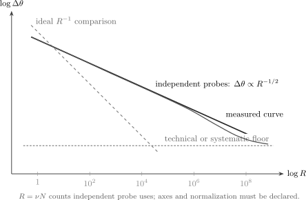
On log–log axes, independent-probe precision has slope $-1/2$. A constant metrological gain moves the curve vertically without changing that exponent. Correlated technical noise or systematics can flatten the observed curve. The ideal $R^{-1}$ line is a comparison, not a promise that an experiment can attain it.

Suppose an uncertainty model is

$$(\Delta\theta)^2 = \frac{A}{R} + B.$$

The first term averages as independent noise. The second is a floor from a correlated fluctuation, calibration uncertainty, or unresolved systematic. The crossover occurs near

$$R_\times = \frac{A}{B}.$$

Below $R_\times$, a log–log fit may look SQL-like. Above it, collecting more probes produces little improvement.

Three claim types must be separated:

• SQL scaling: an exponent compatible with $R^{-1/2}$;
• sub-SQL constant: lower variance than a matched independent-probe benchmark at a specified $R$;
• super-classical scaling: an exponent better than $-1/2$ over a justified range.

A state can provide a useful constant-factor gain while retaining $R^{-1/2}$ asymptotic scaling. Conversely, a fitted steep slope over a narrow pre-asymptotic interval does not establish a new asymptotic law.

What Beating the SQL Means

For the normalized phase problem, define a metrological noise parameter

$$\xi^2 = \nu N (\Delta\theta)^2.$$

The independent-probe benchmark has $\xi^2\ge1$. A measured value

$$\xi^2<1$$

supports sub-SQL performance only if the same losses, duration, prior, estimator, and accepted-run rule are used for the quantum strategy and comparator.

For collective spins, the Wineland squeezing parameter is

$$\xi_R^2 = \frac{ N(\Delta J_\perp)^2 }{ \left| \langle\mathbf J\rangle \right|^2 },$$

with the transverse direction and phase response chosen consistently. $\xi_R^2<1$ certifies a phase sensitivity below the coherent-spin-state benchmark under those conventions.

For $N$ qubits and a collective linear generator, the condition

$$F_Q[\rho,J_{\mathbf n}] > N$$

implies that $\rho$ is entangled and has sub-SQL potential for that local estimation problem. This does not guarantee that an available measurement attains the QFI, that the advantage survives loss, or that the full sensor outperforms a classical instrument.

The SQL Is Not a Universal Quantum Bound

It is not the Heisenberg uncertainty relation

The SQL is an estimation benchmark for a strategy class. The Robertson uncertainty relation constrains variances of two observables in one state. One cannot derive a complete sensor limit merely by inserting a position–momentum or number–phase slogan.

Entanglement can change the ideal scaling

Entangled probes can have QFI proportional to $N^2$ in noiseless local models, suggesting

$$\Delta\theta \propto \frac{1}{N\sqrt\nu}.$$

That ideal Heisenberg scaling requires careful counting of generator range, channel uses, interactions, time, and prior information. It also does not imply an end-to-end advantage.

Noise can restore inverse-square-root scaling

For many common independent loss and decoherence models, asymptotically optimal quantum strategies retain at most a constant-factor advantage over $N^{-1/2}$ scaling. This is a broad and important result, not a universal theorem for every correlated, non-Markovian, error-corrected, or controlled sensing model. The noise channel and available controls decide the bound.

Classical improvements can beat a weak baseline

Feedback, a better estimator, more complete likelihood, higher collection efficiency, longer interrogation, or a better operating point can outperform an earlier “shot-noise” number without using a nonclassical probe. The correct comparator is the best allowed independent-probe strategy under matched resources, not a convenient historical implementation.

Continuous-Measurement SQL Is Different

In a weak continuous position measurement, increasing measurement strength can reduce imprecision while increasing force backaction. A generic added displacement-noise spectrum has the structure

$$\begin{aligned} S_{xx}^{\mathrm{add}}(\omega) ={}& S_{xx}^{\mathrm{imp}}(\omega) + \left| \chi(\omega) \right|^2 S_{FF}^{\mathrm{BA}}(\omega) \\ &+ 2\operatorname{Re} \left[ \chi(\omega) S_{xF}(\omega) \right], \end{aligned}$$

where $\chi$ is the mechanical susceptibility, $S_{xx}^{\mathrm{imp}}$ is measurement imprecision, $S_{FF}^{\mathrm{BA}}$ is backaction-force noise, and $S_{xF}$ contains correlations.

Under a particular uncorrelated quantum-limited detector model, minimizing the first two terms produces a frequency-dependent SQL. Correlations, variational readout, backaction evasion, or a quantum nondemolition observable can alter that optimum. This spectral tradeoff is conceptually related to quantum estimation but is not the $\nu N$ independent-probe SQL derived above.

How to Audit an SQL Claim

A statement such as “3 dB below the SQL” should answer:

Audit item	Required information
estimated parameter	phase, frequency, displacement, field, loss, time, or another quantity
risk	variance, mean-square error, Allan deviation, spectral density, or confidence width
benchmark class	coherent light, separable spins, product qubits, or a continuous detector model
resources	incident and detected probes, energy, passes, time, bandwidth, and duty cycle
loss boundary	where efficiency enters and whether discarded events count
operating regime	local phase point, prior, dynamic range, and estimator calibration
evidence	raw statistics, uncertainty on the gain, scaling range, and noise decomposition
implementation	state preparation, readout, technical noise, drift, and postselection

If variances are compared, a gain factor can be written

$$G = \frac{ (\Delta\theta_{\mathrm{SQL}})^2 }{ (\Delta\theta_{\mathrm{test}})^2 }.$$

The gain in decibels is

$$G_{\mathrm{dB}} = 10\log_{10}G.$$

A positive value is meaningful only relative to the declared benchmark and boundary. Claims, Hype, and Evidence Standards supplies the wider evidence framework.

Common Mistakes

Calling every $1/\sqrt N$ law quantum

Inverse-square-root averaging is a statistical structure. It becomes a quantum limit only after the irreducible one-probe distribution and allowed strategy class are specified.

Omitting the single-probe prefactor

The general bound contains $F_Q^{(1)}$. Writing $1/\sqrt N$ silently chooses units and a normalized generator.

Comparing detected probes with incident probes

Loss and postselection must be charged consistently to both strategies.

Treating variance as Fisher information for mixed states

Classical mixtures can have large generator variance while carrying no parameter dependence.

Equating a constant gain with Heisenberg scaling

A curve proportional to $0.7/\sqrt N$ beats a unit-prefactor SQL but still has SQL scaling.

Ignoring estimator bias and prior knowledge

A constant estimator can have zero variance and no information. Cramér–Rao statements require local unbiasedness or a bias-aware generalization.

Treating a quiet sensor as an accurate sensor

Statistical precision does not remove calibration bias or systematic uncertainty.

Using “SQL” without naming which one

Independent probes, optical shot noise, spin projection noise, and continuous measurement have related but distinct bounds.

Exercises

1. Fisher information of a binary fringe

For

$$p_\pm(\theta) = \frac{1\pm\sin\theta}{2},$$

show that one probe has $F_C^{(1)}=1$. What precision bound follows for $R$ independent probes?

Solution

The derivatives are

$$\partial_\theta p_\pm = \pm\frac{\cos\theta}{2}.$$

Hence

$$\begin{aligned} F_C^{(1)} &= \frac{\cos^2\theta}{4} \left( \frac{1}{p_+} + \frac{1}{p_-} \right) \\ &= \frac{\cos^2\theta}{4} \frac{p_++p_-}{p_+p_-} \\ &= 1, \end{aligned}$$

because $p_+p_-=\cos^2\theta/4$. The result extends to the endpoints by a limit. Additivity gives $F_C^{(R)}=R$, so a locally unbiased estimator satisfies

$$\Delta\theta \ge \frac{1}{\sqrt R}.$$

2. Additivity for independent likelihoods

Let $X_1,\ldots,X_R$ be independent with one-probe score

$$s_j = \partial_\theta \log p(X_j\mid\theta).$$

Show that the total Fisher information is $R F_C^{(1)}$ under the usual regularity condition $\mathbb E[s_j]=0$.

Solution

The joint score is

$$S = \sum_{j=1}^{R}s_j.$$

Therefore

$$\mathbb E[S^2] = \sum_j \mathbb E[s_j^2] + \sum_{j\ne k} \mathbb E[s_js_k].$$

Independence and zero mean give

$$\mathbb E[s_js_k] = \mathbb E[s_j]\mathbb E[s_k] = 0$$

for $j\ne k$. Each diagonal term is $F_C^{(1)}$, so

$$F_C^{(R)} = \mathbb E[S^2] = R F_C^{(1)}.$$

3. Coherent-spin SQL

A coherent spin state has $\langle J_x\rangle=N/2$ and $(\Delta J_y)^2=N/4$. A small $z$ rotation gives $\partial_\theta\langle J_y\rangle=N/2$. Derive the one-round phase uncertainty and evaluate it for $N=10^6$.

Solution

Error propagation gives

$$\Delta\theta = \frac{ \sqrt{N}/2 }{ N/2 } = \frac{1}{\sqrt N}.$$

For $N=10^6$,

$$\Delta\theta = 10^{-3}\ \mathrm{rad}$$

in the ideal local model.

4. Detection efficiency

An experiment sends $R_{\mathrm{in}}=10^8$ independent normalized probes and has efficiency $\eta=0.64$. Find the detection-limited SQL if no information is obtained from lost probes. Compare it with the incorrectly loss-free value.

Solution

The expected detected resource is

$$R_{\mathrm{det}} = 0.64\times10^8 = 6.4\times10^7.$$

Thus

$$\Delta\theta_{\mathrm{SQL}} \gtrsim \frac{1}{\sqrt{6.4\times10^7}} = 1.25\times10^{-4}.$$

Ignoring loss would give $10^{-4}$. The loss increases the uncertainty by $1/\sqrt{0.64}=1.25$.

5. Statistical-to-floor crossover

Suppose

$$(\Delta\theta)^2 = \frac{10^{-2}}{R} + 10^{-10}.$$

Find the resource $R_\times$ where the two contributions are equal and the asymptotic uncertainty floor.

Solution

Set the two variance terms equal:

$$\frac{10^{-2}}{R_\times} = 10^{-10}.$$

Therefore

$$R_\times = 10^8.$$

For $R\gg10^8$, the variance approaches $10^{-10}$, so the standard deviation approaches

$$\Delta\theta_{\mathrm{floor}} = 10^{-5}.$$

6. A variance trap

For

$$\rho = \frac12 |0\rangle\langle0|^{\otimes N} + \frac12 |1\rangle\langle1|^{\otimes N},$$

compute $(\Delta J_z)^2$ and explain why the state has zero QFI for a $J_z$-generated phase.

Solution

The two components have $J_z$ eigenvalues $+N/2$ and $-N/2$. The mean is zero and

$$(\Delta J_z)^2 = \frac12 \left( \frac N2 \right)^2 + \frac12 \left( -\frac N2 \right)^2 = \frac{N^2}{4}.$$

Nevertheless, $\rho$ is diagonal in the $J_z$ basis, so

$$e^{-i\theta J_z} \rho e^{i\theta J_z} = \rho.$$

No measurement can infer $\theta$ from an unchanged state, and $F_Q[\rho,J_z]=0$. For mixed states, generator variance can be classical rather than phase-sensitive.

7. Constant gain versus scaling gain

A protocol achieves

$$\Delta\theta = \frac{0.8}{\sqrt R}.$$

Does it beat the unit-prefactor SQL? Does it exhibit Heisenberg scaling? Compute its variance gain in decibels.

Solution

At matched $R$, its variance is $0.64/R$ rather than $1/R$, so it beats the unit-prefactor SQL by

$$G = \frac{1}{0.64} = 1.5625.$$

The decibel gain is

$$G_{\mathrm{dB}} = 10\log_{10}(1.5625) \approx 1.94\ \mathrm{dB}.$$

Its exponent remains $-1/2$, so this is a constant-factor sub-SQL gain, not Heisenberg scaling.

8. Count multiple passes

$R$ probes each pass through a phase sample $m$ times, producing a local phase response $m$ times larger than a single pass. The raw error propagation gives $\Delta\theta=1/(m\sqrt R)$. Express this in terms of the total channel uses $R_{\mathrm{use}}=mR$.

Solution

Since $R=R_{\mathrm{use}}/m$,

$$\Delta\theta = \frac{1}{ m\sqrt{R_{\mathrm{use}}/m} } = \frac{1}{ \sqrt{ mR_{\mathrm{use}} } }.$$

At fixed pass number $m$, the scaling with total channel uses remains $R_{\mathrm{use}}^{-1/2}$, though the prefactor improves. If $m$ itself grows with the resource, interrogation time, loss, and sample exposure must also be included before assigning a scaling class.

9. Why unbiasedness matters

The estimator $\widehat\theta=0$ has zero variance for every data set. Why does it not violate the Cramér–Rao bound for an unknown $\theta$?

Solution

Its expectation is always zero, so its bias is

$$b(\theta) = \mathbb E_\theta[\widehat\theta]-\theta = -\theta.$$

It is not locally unbiased except at a single point under a weak interpretation, and it has mean-square error

$$\mathbb E_\theta[ (\widehat\theta-\theta)^2 ] = \theta^2.$$

Variance alone is not a valid risk for comparing arbitrarily biased estimators. One must use an unbiased or bias-aware bound, a local minimax risk, or a Bayesian risk with a declared prior.

10. Audit a sub-SQL claim

An experiment reports “4 dB below the SQL” after discarding 70% of runs and compares its accepted events with a benchmark charged for every input probe. Identify the principal defect and state a fair comparison.

Solution

The postselection boundaries do not match. The test strategy reports conditional performance per accepted event, while the benchmark pays for all attempts. A fair comparison must apply the same acceptance rule or charge both strategies for total incident probes, elapsed time, failed runs, and any heralding resources.

The report should also give the estimator risk, uncertainty on the 4 dB number, loss and detector efficiencies, technical-noise subtraction, operating point, and whether discarded outcomes could depend on the unknown parameter.

References

1. H. Cramér, Mathematical Methods of Statistics, Princeton University Press (1946), publisher record.
2. C. R. Rao, “Information and the accuracy attainable in the estimation of statistical parameters,” Bulletin of the Calcutta Mathematical Society 37, 81–91 (1945), reprint doi:10.1007/978-1-4612-0919-5_16.
3. C. W. Helstrom, Quantum Detection and Estimation Theory, Academic Press (1976), doi:10.1016/C2013-0-10310-8.
4. S. L. Braunstein and C. M. Caves, “Statistical distance and the geometry of quantum states,” Physical Review Letters 72, 3439–3443 (1994), doi:10.1103/PhysRevLett.72.3439.
5. C. M. Caves, “Quantum-mechanical noise in an interferometer,” Physical Review D 23, 1693–1708 (1981), doi:10.1103/PhysRevD.23.1693.
6. B. Yurke, S. L. McCall, and J. R. Klauder, “SU(2) and SU(1,1) interferometers,” Physical Review A 33, 4033–4054 (1986), doi:10.1103/PhysRevA.33.4033.
7. D. J. Wineland, J. J. Bollinger, W. M. Itano, F. L. Moore, and D. J. Heinzen, “Spin squeezing and reduced quantum noise in spectroscopy,” Physical Review A 46, R6797–R6800 (1992), doi:10.1103/PhysRevA.46.R6797.
8. V. Giovannetti, S. Lloyd, and L. Maccone, “Quantum-enhanced measurements: Beating the standard quantum limit,” Science 306, 1330–1336 (2004), doi:10.1126/science.1104149.
9. V. Giovannetti, S. Lloyd, and L. Maccone, “Quantum metrology,” Physical Review Letters 96, 010401 (2006), doi:10.1103/PhysRevLett.96.010401.
10. S. F. Huelga et al., “Improvement of frequency standards with quantum entanglement,” Physical Review Letters 79, 3865–3868 (1997), doi:10.1103/PhysRevLett.79.3865.
11. B. M. Escher, R. L. de Matos Filho, and L. Davidovich, “General framework for estimating the ultimate precision limit in noisy quantum-enhanced metrology,” Nature Physics 7, 406–411 (2011), doi:10.1038/nphys1958.
12. R. Demkowicz-Dobrzański, J. Kołodyński, and M. Guţă, “The elusive Heisenberg limit in quantum-enhanced metrology,” Nature Communications 3, 1063 (2012), doi:10.1038/ncomms2067.
13. L. Pezzè, A. Smerzi, M. K. Oberthaler, R. Schmied, and P. Treutlein, “Quantum metrology with nonclassical states of atomic ensembles,” Reviews of Modern Physics 90, 035005 (2018), doi:10.1103/RevModPhys.90.035005.
14. A. A. Clerk, M. H. Devoret, S. M. Girvin, F. Marquardt, and R. J. Schoelkopf, “Introduction to quantum noise, measurement, and amplification,” Reviews of Modern Physics 82, 1155–1208 (2010), doi:10.1103/RevModPhys.82.1155.
15. M. G. A. Paris, “Quantum estimation for quantum technology,” International Journal of Quantum Information 7, 125–137 (2009), doi:10.1142/S0219749909004839.
16. G. Tóth and I. Apellaniz, “Quantum metrology from a quantum information science perspective,” Journal of Physics A 47, 424006 (2014), doi:10.1088/1751-8113/47/42/424006.
17. L. Pezzè and A. Smerzi, “Entanglement, nonlinear dynamics, and the Heisenberg limit,” Physical Review Letters 102, 100401 (2009), doi:10.1103/PhysRevLett.102.100401.

Further Connections

• Quantum Measurement as Estimation develops the estimation contract that must be fixed before a precision benchmark can be interpreted.
• Quantum Illumination treats binary target-channel discrimination, whose coherent-state benchmark and error exponent should not be relabeled as an SQL precision law.
• Classical and Quantum Fisher Information derives the SLD metric, optimal-measurement bound, state formulas, and compatibility caveats used here.
• Cramér–Rao Bounds owns the unbiasedness, regularity, nuisance-parameter, and attainability conditions behind the variance bounds used here.
• Heisenberg Scaling develops the ideal inverse-resource law, global phase ambiguity, nonlinear encodings, and noise-induced crossovers.
• Squeezing develops response-aware noise reduction, covariance geometry, loss, and the distinction between a constant gain and a changed scaling exponent.
• Spin Squeezing turns the coherent-spin projection-noise reference into the Kitagawa–Ueda and Wineland parameters used in ensemble metrology.
• Ramsey Interferometry realizes the independent-probe benchmark as a binary fringe and adds contrast, interrogation time, aliases, and duty cycle.
• Mach–Zehnder Interferometry turns optical shot noise into a matched-resource comparison across incident, interacting, absorbed, detected, and reference photons.
• Atomic Clocks converts projection noise into information per wall time and tests the benchmark inside a noisy oscillator-tracking loop.
• Gravimetry and Inertial Sensing constructs the matched independent-atom benchmark for accelerometers, gravimeters, gyroscopes, and gradiometers, including accepted-shot and cycle-time resources.
• Distributed Quantum Sensing distinguishes product-probe, locally entangled node-separable, and inter-node-entangled bounds for weighted spatial parameters.
• Fisher Information derives scores, additivity, reparameterization, and the classical Cramér–Rao bound.
• Variance and Covariance supplies the independent-sum and error-propagation identities used here.
• GHZ States provide the canonical ideal state with collective-generator variance proportional to $N^2$.
• Squeezed Light owns optical source physics, mode definitions, homodyne calibration, and detector-plane loss.
• Precision Measurement and Metrology connects projection-noise scaling to clocks, interferometers, and real instrument budgets.
• Quantum Information Roadmap places sensing after states, channels, measurements, and estimation theory.