Gravimetry and Inertial Sensing

An atom-interferometric inertial sensor converts motion relative to an optical phase reference into a matter-wave phase and then into atomic output populations. With ideal light pulses, a uniform acceleration produces the familiar phase

$$\Phi_a = \mathbf k_{\mathrm{eff}} \mathbin{\cdot} \mathbf a_{\mathrm{rel}}T^2.$$

The same apparatus can act as a gravimeter, accelerometer, gyroscope, or gradiometer, but those are different estimation tasks. They use different response vectors, references, nuisance models, spatial baselines, and validation data. A narrow phase distribution is not yet an accurate gravity measurement, and an entangled atomic source is not yet a quantum-enhanced inertial sensor.

This page is the canonical home for the quantum-estimation and quantum-resource layer of gravimetry and inertial sensing. It develops the population likelihood, Fisher matrix, phase ambiguity, matched independent- atom benchmark, transfer of squeezing through a matter-wave sequence, information per wall time, multiparameter identifiability, hybrid sensing, and evidence required for a quantum-enhancement claim.

Atom Interferometry owns Raman and Bragg beam splitters, phase bookkeeping, sensitivity functions, wave-packet closure, contrast, and state-selective readout. Atom-Interferometric Sensors owns the detailed instrument layer: absolute-gravity conventions, reference height, geophysical corrections, gradient and rotation calibration, wavefront and Coriolis shifts, covariance budgets, reversals, and field validation. Sensing Case Studies retains the historical evidence narrative for a transportable gravimeter.

Define the Estimation Task

One experimental configuration $j$ can be represented locally by

$$\Phi_j = \mathbf K_{a,j} \mathbin{\cdot} \mathbf a + \mathbf K_{\Omega,j} \mathbin{\cdot} \boldsymbol\Omega + \mathbf K_{\Gamma,j} : \boldsymbol\Gamma +b_j.$$

Here $\mathbf a$ is an acceleration parameter, $\boldsymbol\Omega$ is angular velocity, $\boldsymbol\Gamma$ is a gravity-gradient or acceleration-gradient tensor, and $b_j$ collects modeled nuisance phases. The double contraction is

$$\mathbf K_{\Gamma,j}:\boldsymbol\Gamma = \sum_{m,n} (K_{\Gamma,j})_{mn}\Gamma_{mn}.$$

A complete sensing contract may be written

$$\mathcal S_{\mathrm I} = (\boldsymbol\theta,\rho, \mathcal C,\mathcal M, \mathbf H,\mathcal E,\mathcal R),$$

where

• $\boldsymbol\theta$ contains the intended inertial parameters and nuisance quantities;
• $\rho$ is the atomic input state, including correlations;
• $\mathcal C$ is the preparation and light-pulse sequence;
• $\mathcal M$ is the population, image, or collective-spin likelihood;
• $\mathbf H$ contains calibrated response vectors and tensors;
• $\mathcal E$ is the estimator, prior information, wrap logic, and uncertainty statement; and
• $\mathcal R$ is the resource ledger: atom numbers at declared boundaries, momentum transfer, interrogation and cycle times, acceptance probability, optical references, and auxiliary sensors.

Changing the task changes the meaning of the data. In a laboratory gravimeter, the atoms are approximately free test masses while a mirror fixed to the ground defines the optical phase. On a vehicle, the same relative acceleration must be combined with attitude and a gravity model to infer platform specific force. In a gyroscope, launch velocity and path area enter the rotation scale factor. In a gradiometer, two response-weighted locations and their baseline define a spatial derivative.

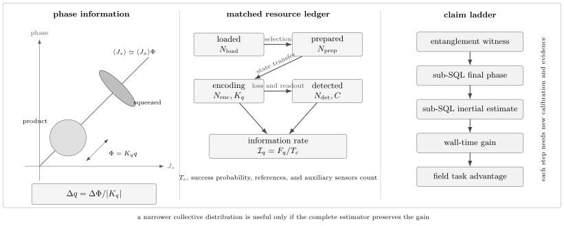
A quantum-enhanced inertial claim has three linked layers. A correlated input must reduce phase uncertainty after the complete interferometer; the inertial response $K_q$ must convert that phase gain into the declared quantity; and the resource ledger must preserve an information-rate or task-level gain after loss, contrast, preparation time, rejected cycles, references, and auxiliary sensors are counted.

Two-Mode Quantum Description

Collective path pseudospin

Let modes $a$ and $b$ denote the two interferometer alternatives, which may combine internal and momentum labels. Define Schwinger collective operators

$$\begin{aligned} J_x &= \frac12 (a^\dagger b+b^\dagger a),\\ J_y &= \frac{1}{2i} (a^\dagger b-b^\dagger a),\\ J_z &= \frac12 (a^\dagger a-b^\dagger b). \end{aligned}$$

For fixed atom number $N$, the total spin is $J=N/2$. Beam splitters rotate this collective spin, relative evolution encodes phase, and the final population difference measures a rotated component. With an appropriate choice of axes, the signal unitary is

$$U_\Phi = e^{-i\Phi G},$$

where $G$ is the generator conjugate to the phase. For an ordinary two-mode linear interferometer, $G$ is one collective-spin component.

At a midfringe operating point, the mean output is locally

$$\langle J_{z,\mathrm{out}}\rangle \simeq \langle J_x\rangle\Phi.$$

Error propagation gives

$$(\Delta\Phi)^2 = \frac{ \operatorname{Var}(J_{z,\mathrm{out}}) }{ |\langle J_x\rangle|^2 }.$$

This expression includes both noise and response slope. Reducing a population variance while destroying coherence need not improve phase estimation.

Independent-atom likelihood

For $N$ independent detected atoms and a balanced two-port readout, a useful fringe model is

$$p(\Phi) = \frac12 \left[ 1+C\sin\Phi \right],$$

with count likelihood

$$n \sim \operatorname{Binomial} \left[N,p(\Phi)\right].$$

The phase Fisher information is

$$F_\Phi = N \frac{ C^2\cos^2\Phi }{ 1-C^2\sin^2\Phi }.$$

At midfringe,

$$F_\Phi(0) = NC^2,$$

and a locally unbiased estimator obeys

$$\Delta\Phi \geq \frac{1}{C\sqrt N}.$$

$C<1$ can represent imperfect state preparation, mode overlap, pulse efficiency, dephasing, and inhomogeneous phase. Detection noise and atom-number fluctuations require a more complete likelihood; they should not be silently absorbed into a fitted contrast if their statistics are distinguishable.

From Phase Information to Inertial Information

Scalar response

If one parameter $q$ produces

$$\Phi(q) = K_q q+b,$$

then Fisher information transforms as

$$F_q = K_q^2F_\Phi.$$

For constant acceleration in the ideal three-pulse geometry,

$$K_a = k_{\mathrm{eff}}T^2,$$

so the independent-atom statistical baseline is

$$\Delta a_{\mathrm{SQL}} \geq \frac{1}{ k_{\mathrm{eff}}T^2C\sqrt N }.$$

For a rotation component along the response vector,

$$\mathbf K_\Omega = 2T^2 \left( \mathbf k_{\mathrm{eff}} \mathbin{\times} \mathbf v \right),$$

and the same phase uncertainty becomes

$$\Delta\Omega_e \geq \frac{1}{ K_\Omega C\sqrt N }.$$

Entanglement changes the phase-information term. It does not calibrate $k_{\mathrm{eff}}$, $T$, launch velocity, beam direction, baseline, or the reference frame.

Vector identifiability

Collect the local phase models into

$$\boldsymbol\Phi = \mathbf H\boldsymbol\theta + \mathbf b.$$

If outcomes from configuration $j$ provide scalar phase information $F_{\Phi,j}$, the parameter Fisher matrix is

$$\mathbf F_{\theta} = \sum_j F_{\Phi,j} \mathbf h_j\mathbf h_j^{\mathsf T},$$

where $\mathbf h_j^{\mathsf T}$ is row $j$ of $\mathbf H$. A single phase channel contributes a rank-one matrix no matter how entangled its atoms are. Recovering three acceleration components, three rotations, or selected gradient components requires enough independent response directions and a well-conditioned nuisance model.

For a linear Gaussian phase estimate with covariance $\boldsymbol\Sigma_\Phi$,

$$\mathbf F_\theta = \mathbf H^{\mathsf T} \boldsymbol\Sigma_\Phi^{-1} \mathbf H.$$

Small singular values of $\mathbf H$ amplify statistical noise and calibration errors. Adding a very precise but nearly redundant axis can contribute little useful information.

The Sensed Temporal Mode

For ideal pulses at $0$, $T$, and $2T$, define

$$f(t) = \begin{cases} t, & 0<t<T,\\ 2T-t, & T<t<2T,\\ 0, & \text{otherwise}. \end{cases}$$

The acceleration phase is

$$\Phi_a = k_{\mathrm{eff}} \int_0^{2T} f(t)a_{\mathrm{rel}}(t)\,dt.$$

It is useful to define the normalized estimand

$$a_f = \frac{1}{T^2} \int_0^{2T} f(t)a_{\mathrm{rel}}(t)\,dt,$$

so that $\Phi_a=k_{\mathrm{eff}}T^2a_f$. The instrument measures this weighted mode, not instantaneous acceleration at the middle pulse. Finite pulses and real control waveforms alter the kernel.

For Fourier convention $a(t)=\int\widetilde a(\omega)e^{-i\omega t}d\omega/(2\pi)$, the ideal transfer function is

$$H_a(\omega) = k_{\mathrm{eff}} e^{-i\omega T} \left[ \frac{2\sin(\omega T/2)}{\omega} \right]^2.$$

This transfer function determines vibration coupling and which auxiliary- sensor frequencies matter. The detailed derivation, finite-pulse correction, cycle aliasing, and spectral-density conventions belong to Atom-Interferometric Sensors.

Periodicity, Priors, and Dynamic Range

The population likelihood is periodic:

$$p(\Phi+2\pi m) = p(\Phi), \qquad m\in\mathbb Z.$$

An ideal acceleration fringe therefore spans

$$\Delta a_{2\pi} = \frac{2\pi}{K_a}.$$

Local Fisher information assumes the correct fringe branch and a known operating point. It does not solve the global estimation problem. With prior $\pi_0(a)$ and data $D$, a posterior has the schematic form

$$p(a|D) \propto p(D|a)\pi_0(a),$$

and can remain multimodal with peaks separated by $2\pi/K_a$. Chirp locking, quadrature channels, several interrogation times, or a mechanical accelerometer can identify the branch. Those references and preliminary measurements are part of the protocol.

Squeezing makes this issue more acute when the operating point is uncertain. If the noise ellipse has squeezed and antisqueezed variances $V_-$ and $V_+$, a phase error $\delta$ rotates both into the readout:

$$V(\delta) = V_-\cos^2\delta + V_+\sin^2\delta.$$

A large $V_+/V_-$ can erase the gain under modest vibration or phase-reference error. Useful protocols stabilize the phase, adapt the readout angle, use states with wider dynamic range, or combine coarse and fine sensors.

Quantum Resources for Inertial Phase

Metrological squeezing

For a collective readout with $N$ atoms, define the operational Wineland parameter

$$\xi_R^2 = N \frac{ \operatorname{Var}(J_{z,\mathrm{out}}) }{ |\partial_\Phi \langle J_{z,\mathrm{out}}\rangle|^2 }.$$

At midfringe, the denominator is $|\langle J_x\rangle|^2$. The attained phase variance is

$$(\Delta\Phi)^2 = \frac{\xi_R^2}{N}.$$

Thus, for the same inertial response,

$$(\Delta q)^2 = \frac{\xi_R^2}{NK_q^2}.$$

$\xi_R^2<1$ certifies metrologically useful squeezing relative to the declared independent-atom boundary under the usual collective-spin assumptions. It includes the contrast penalty through the response slope. Noise squeezing alone, for example

$$\frac{4\operatorname{Var}(J_z)}{N}<1,$$

does not guarantee $\xi_R^2<1$ if coherence is lost.

An enhancement in decibels is commonly reported as

$$G_{\mathrm{dB}} = -10\log_{10}\xi_R^2.$$

A $3\ \mathrm{dB}$ gain halves variance and reduces standard deviation by $\sqrt2$; it does not reduce standard deviation by a factor of two.

Quantum Fisher information

For a pure state encoded by $U_\Phi=e^{-i\Phi G}$,

$$F_Q(\Phi) = 4\operatorname{Var}(G).$$

With the conventional normalization in which each independent two-mode atom has a unit maximum phase Fisher information, separable inputs obey

$$F_Q(\Phi) \leq N.$$

Entangled states can have $F_Q>N$, and ideal maximally correlated states can reach order $N^2$. For inertial parameter $q$,

$$F_Q(q) = K_q^2F_Q(\Phi).$$

This is a local bound. A laboratory still needs a measurement that attains the information, a prior narrow enough to avoid phase aliases, and robustness to loss and phase diffusion. Classical and Quantum Fisher Information owns the general optimization, while Heisenberg Scaling owns the resource and global-estimation caveats behind ideal $1/N$ laws.

Ways to create useful correlations

Several architectures can supply nonclassical matter-wave inputs:

• collisional spin mixing can create twin-Fock or two-mode squeezed states, followed by coherent transfer from internal to momentum modes;
• one-axis twisting can shear a collective uncertainty distribution into a spin-squeezed state;
• cavity-mediated interactions can generate correlations while mode-filtered cavity fields drive or read momentum transitions; and
• quantum nondemolition measurements can condition or feedback-stabilize a reduced collective variance.

The entangled degree of freedom must match the generator and detector. Internal spin squeezing that is lost during momentum mapping does not enhance a spatial interferometer. Conversely, a squeezed momentum population can survive release yet fail to improve the final phase if recombination contrast or readout slope is degraded.

Match the Resource Boundary

Atom and time ledgers

At least four atom numbers may differ:

$$N_{\mathrm{load}} \geq N_{\mathrm{prep}} \geq N_{\mathrm{enc}} \geq N_{\mathrm{det}}.$$

$N_{\mathrm{enc}}$ counts atoms that enter the phase-encoding sequence in the declared state. A benchmark using $N_{\mathrm{det}}$ for the correlated protocol but $N_{\mathrm{enc}}$ for the product protocol is mismatched. Other resources include

$$\mathcal R = \left( N_{\mathrm{enc}}, k_{\mathrm{eff}},T,T_c, C,q_{\mathrm{acc}}, P_{\mathrm{opt}}, \mathcal A_{\mathrm{aux}} \right),$$

where $T_c$ is cycle time, $q_{\mathrm{acc}}$ is acceptance probability, $P_{\mathrm{opt}}$ summarizes relevant optical resources, and $\mathcal A_{\mathrm{aux}}$ denotes auxiliary sensors and references.

For independent white cycles, define information rate

$$\mathcal I_q = \frac{F_q}{T_c}.$$

Equivalently, if the one-cycle standard deviation is $\sigma_q$, the noise-equivalent sensitivity is

$$\eta_q = \sigma_q\sqrt{T_c},$$

so that $\sigma_q(\tau)\simeq\eta_q/\sqrt\tau$. A fair wall-time gain is

$$G_{\mathrm{rate}} = \frac{ F_{q,\mathrm{sq}}/T_{c,\mathrm{sq}} }{ F_{q,\mathrm{prod}}/T_{c,\mathrm{prod}} }.$$

A $3\ \mathrm{dB}$ per-shot variance gain is exactly canceled if squeezing doubles the cycle time while all other resources remain equal.

Acceptance and postselection

If a preparation succeeds with probability $q(\theta)$ and both accepted and rejected records are retained, the Fisher information per attempt can be decomposed as

$$F_{\mathrm{tot}} = qF_{\mathrm{acc}} + (1-q)F_{\mathrm{rej}} + \frac{ [\partial_\theta q]^2 }{q(1-q)}.$$

When $q$ is parameter independent and rejected trials carry no information, $F_{\mathrm{tot}}=qF_{\mathrm{acc}}$. Reporting only $F_{\mathrm{acc}}$ overstates performance. The clock continues to run while an entangled state fails to prepare.

Technical-noise crossover

Suppose a matched product state has quantum phase variance $1/N$, a squeezed state has $\xi_R^2/N$, and both share additive technical variance $\sigma_{\mathrm{tech}}^2$. Then

$$\begin{aligned} \sigma_{\Phi,\mathrm{prod}}^2 &= \frac1N+\sigma_{\mathrm{tech}}^2,\\ \sigma_{\Phi,\mathrm{sq}}^2 &= \frac{\xi_R^2}{N} +\sigma_{\mathrm{tech}}^2. \end{aligned}$$

The total variance gain is

$$G_{\mathrm{tot}} = \frac{ N^{-1}+\sigma_{\mathrm{tech}}^2 }{ \xi_R^2N^{-1}+\sigma_{\mathrm{tech}}^2 }.$$

As vibration, laser phase noise, wavefront variation, or detection noise dominates, $G_{\mathrm{tot}}\to1$. Quantum enhancement is most useful after technical noise has been suppressed below or near the independent-atom term.

Loss, Contrast, and Interactions

Particle loss reduces atom number and can destroy correlations. Detection inefficiency is not equivalent to losing atoms before phase encoding: the latter changes the state that senses the parameter, while the former discards outcomes after encoding. A resource audit should locate each loss.

Strongly correlated states have different fragilities. An $N$-atom GHZ-like coherence can be destroyed by one lost atom in a simple loss model, giving a survival factor that scales as

$$P_{\mathrm{coh}} \sim \eta^N.$$

Moderately squeezed states often degrade more gracefully, but their actual gain depends on loss channel, generator, and readout. There is no universal formula obtained by replacing $N$ with $\eta N$.

Interactions can both create squeezing and produce unwanted phase diffusion, density shifts, mode deformation, and expansion. A Bose–Einstein condensate offers low expansion and high mode quality, yet its source cycle can be long and its mean-field dynamics must be controlled. Delta-kick collimation can reduce expansion without being an entanglement resource. Improvements from larger $k_{\mathrm{eff}}$, longer $T$, colder atoms, higher flux, better contrast, or better vibration rejection are valuable but should be named as response or engineering gains rather than attributed to entanglement.

Differential and Rotation Measurements

Gradiometry

Let two interferometers estimate phases $\Phi_1$ and $\Phi_2$. The differential phase is

$$\Delta\Phi = \Phi_2-\Phi_1.$$

Its variance is

$$\operatorname{Var}(\Delta\Phi) = V_1+V_2-2\operatorname{Cov}(\Phi_1,\Phi_2).$$

For independent product states with equal atom number $N$, contrast $C$, and negligible technical noise,

$$\operatorname{Var}(\Delta\Phi)_{\mathrm{SQL}} = \frac{2}{C^2N}.$$

Common optical-phase or vibration noise can produce useful classical covariance and cancel in the difference. Local squeezing can reduce $V_1$ and $V_2$. Entanglement shared between sensor nodes can instead engineer the differential quadrature directly. These strategies have different resource boundaries and robustness; a common-mode rejection ratio is not itself proof of nonclassical enhancement.

For effective baseline $L_{\mathrm{eff}}$ and matched acceleration scale factor,

$$\widehat\Gamma = \frac{ \Delta\Phi-\Delta b }{ k_{\mathrm{eff}}T^2L_{\mathrm{eff}} }.$$

Quantum correlations do not determine $L_{\mathrm{eff}}$ or eliminate leakage from a common acceleration through scale-factor mismatch.

Rotation and multi-axis sensing

Counterpropagating trajectories can generate phases

$$\begin{aligned} \Phi_+ &= K_a a+K_\Omega\Omega+b_+,\\ \Phi_- &= K_a a-K_\Omega\Omega+b_-. \end{aligned}$$

Their sum and difference separate acceleration-like and rotation-like channels only to the extent that scale factors and trajectories match. Squeezing both channels lowers their quantum statistical terms but cannot correct a launch- velocity drift or wavefront asymmetry.

Simultaneous arrays can provide several response vectors in one shot. Their advantage over sequential axis rotation is reduced temporal mismatch, not automatic rank or calibration. A multi-axis quantum-enhancement claim should compare covariance matrices or a declared scalar loss, for example

$$\mathcal L = \operatorname{Tr} \left( \mathbf W \operatorname{Cov}\widehat{\boldsymbol\theta} \right),$$

with positive task-weight matrix $\mathbf W$, rather than selecting the best single diagonal element after the measurement.

Hybrid Quantum–Classical Inertial Sensing

Atom interferometers usually have excellent low-frequency stability but cyclic readout and limited capture range. Mechanical accelerometers and optical or electromechanical gyroscopes offer higher bandwidth and dynamic range but can have drifting bias. A hybrid estimator uses both data streams.

The correct statistical object is a joint model such as

$$p \left( n_k,z_{\mathrm{aux}}(t) \mid \boldsymbol\theta, \boldsymbol\lambda \right),$$

where $n_k$ is the atomic output and $z_{\mathrm{aux}}(t)$ is the auxiliary record. Gain, delay, axis orientation, lever arm, saturation, and auxiliary bias belong to $\boldsymbol\lambda$. Filtering the auxiliary record through the atomic sensitivity function predicts the vibration phase and often identifies the fringe branch.

An auxiliary sensor can increase usable information by preserving operation in a dynamic environment. It does not reduce atom projection noise, and it is not free. A quantum-enhancement comparison must give product and entangled protocols access to the same auxiliary record, or count any difference as a resource. Field performance should be judged from the final hybrid output, including cycle slips and bias tracking, not from a quiet subset of atomic shots.

Worked Resource Audit

Consider a vertical interferometer with

$$\begin{aligned} k_{\mathrm{eff}} &= 1.61\times10^7\ \mathrm{m^{-1}},\\ T &= 0.100\ \mathrm s,\\ N &= 10^6,\\ C &= 0.40,\\ T_c &= 0.50\ \mathrm s. \end{aligned}$$

The ideal scale factor is

$$K_a = k_{\mathrm{eff}}T^2 = 1.61\times10^5\ \frac{\mathrm{rad}} {\mathrm{m\,s^{-2}}}.$$

The independent-atom phase and acceleration baselines are

$$\Delta\Phi_{\mathrm{SQL}} = \frac{1}{C\sqrt N} = 2.50\times10^{-3}\ \mathrm{rad},$$

and

$$\Delta a_{\mathrm{SQL}} = 1.55\times10^{-8}\ \mathrm{m\,s^{-2}}$$

per cycle. The white-noise coefficient is

$$\eta_a = \Delta a_{\mathrm{SQL}}\sqrt{T_c} = 1.10\times10^{-8}\ \mathrm{m\,s^{-2}\,Hz^{-1/2}}.$$

Now suppose a correlated protocol achieves $3.00\ \mathrm{dB}$ of operational metrological gain, so

$$\xi_R^2 = 10^{-3/10} = 0.501.$$

At unchanged $N$, $C$, and $K_a$, the one-cycle acceleration standard deviation becomes

$$\Delta a_{\mathrm{sq}} = \sqrt{0.501}\, \Delta a_{\mathrm{SQL}} = 1.10\times10^{-8}\ \mathrm{m\,s^{-2}}.$$

If squeezing increases cycle time to $1.00\ \mathrm s$, however,

$$\eta_{a,\mathrm{sq}} = 1.10\times10^{-8}\ \mathrm{m\,s^{-2}\,Hz^{-1/2}},$$

essentially equal to the product-state value. The per-shot gain is real, but there is no gain per wall time in this example. If both protocols also have $2.0\ \mathrm{mrad}$ RMS technical phase noise, the attainable variance gain is only

$$G_{\mathrm{tot}} = \frac{ (2.50\ \mathrm{mrad})^2+(2.0\ \mathrm{mrad})^2 }{ 0.501(2.50\ \mathrm{mrad})^2+(2.0\ \mathrm{mrad})^2 } \simeq 1.44,$$

or $1.58\ \mathrm{dB}$. The rest of the nominal $3\ \mathrm{dB}$ is hidden under shared technical noise.

Experimental Evidence

The evidence has progressed through distinct milestones that should not be treated as equivalent.

Result	What was demonstrated	What remained outside the claim
Anders et al. (2021)	Entanglement was transferred from spin to separated momentum modes; conditional squeezing of $-3.1(8)\ \mathrm{dB}$ was reported.	No acceleration or rotation estimate was improved. This was a source and compatibility demonstration.
Greve et al. (2022)	A 700-atom cavity system injected squeezed external modes into a light-pulse matter-wave sequence and reported $1.7^{+0.5}_{-0.5}\ \mathrm{dB}$ directly observed phase sensitivity below its SQL.	The useful duration was short and the experiment did not establish a calibrated field gravimeter. A 2023 arXiv critique disputed the SQL interpretation; the published article remains the version of record, with only an unrelated publisher correction to figure labels.
Cassens et al. (2025)	A Bose–Einstein-condensate gravimeter measured gravitational acceleration with reported sensitivity $-1.7^{+0.4}_{-0.5}\ \mathrm{dB}$ below the stated SQL. Over the first $800\ \mathrm s$, the squeezed result averaged about $1.4$ times faster than that SQL and $2.2$ times faster than the coherent implementation.	The result was a controlled laboratory demonstration with a long source cycle. It did not establish lower systematic uncertainty, navigation performance, or superiority to the best mature gravimeter under all resources.

The 2025 result is stronger than a squeezing witness because an inertial quantity was estimated and compared with a product-state boundary. It is still not a universal claim that entanglement improves every gravimeter. Mature unentangled atom gravimeters have demonstrated transport, long operation, and careful systematic evaluation. Quantum statistical gain and field readiness are separate axes of evidence.

What Different Claims Establish

Claim	Minimum evidence	Does not by itself establish
entangled source	a valid witness at the relevant resource boundary	interferometric gain
momentum-mode squeezing	correlations survive mapping and spatial separation	final phase sensitivity
sub-SQL phase readout	complete interferometer likelihood beats a matched product-state phase benchmark	calibrated acceleration or gravity
quantum-enhanced acceleration	phase gain survives the same calibrated $K_a$ and estimator	wall-time or field advantage
information-rate gain	total Fisher information per elapsed time improves with failures counted	lower systematic uncertainty
field-ready quantum advantage	final hybrid task loss beats an optimized matched comparator under dynamic conditions	universal superiority

An absolute-gravity uncertainty budget contains beam alignment, frequency and timing, wavefronts, Coriolis effects, gravity gradients, reference height, tides, atmospheric loading, self-attraction, and local mass changes. Squeezing directly addresses none of those biases. It can reduce statistical averaging time, which may indirectly reduce exposure to drift, but that benefit must be measured.

Common Mistakes

Calling every atom interferometer quantum enhanced

Matter-wave interference is quantum mechanical. “Quantum enhanced” requires a matched nonclassical-resource advantage, usually against the best allowed separable atomic protocol.

Using squeezed variance without the response slope

Contrast loss can erase noise reduction. Use $\xi_R^2$ or the measured Fisher information, not number variance alone.

Comparing different atom-number boundaries

Prepared, phase-encoding, surviving, and detected atom numbers are not interchangeable. State the boundary used by both protocols.

Reporting per-shot gain as sensitivity gain

Preparation, cooling, feedback, rejected trials, and dead time determine information per wall time.

Treating local Fisher information as global certainty

One fringe is periodic. A narrow local distribution can coexist with an unknown integer wrap or a wrong branch selected by an auxiliary sensor.

Crediting squeezing for a larger scale factor

Longer $T$ and larger $k_{\mathrm{eff}}$ improve inertial response. They are valuable resources but are not entanglement gain.

Assuming differential cancellation is quantum

Shared laser or vibration noise can cancel classically. A nonclassical claim must isolate the covariance produced by the quantum state and compare it with a matched separable network.

Equating stability with gravity accuracy

A low Allan deviation or sub-SQL statistical term does not validate reference height, wavefront, Coriolis, gradient, or environmental corrections.

Key Results

For an independent-atom fringe at midfringe,

$$F_\Phi = NC^2, \qquad \Delta a_{\mathrm{SQL}} \geq \frac{1}{ k_{\mathrm{eff}}T^2C\sqrt N }.$$

For an operationally squeezed collective readout,

$$(\Delta q)^2 = \frac{\xi_R^2}{NK_q^2}.$$

For several inertial parameters,

$$\mathbf F_\theta = \sum_j F_{\Phi,j} \mathbf h_j\mathbf h_j^{\mathsf T}.$$

The experimentally relevant comparison is often information rate,

$$\mathcal I_q = \frac{F_q}{T_c},$$

with losses, preparation failures, phase references, auxiliary sensors, dynamic range, and systematics included at the same boundary. Entanglement can improve the quantum statistical term. It does not replace the inertial response model or the measurement uncertainty budget.

Further Connections

• Quantum Measurement as Estimation develops estimands, likelihoods, nuisance parameters, estimators, and claim validation.
• Standard Quantum Limit owns the independent-probe benchmark and general resource audit.
• Spin Squeezing derives the Wineland parameter, contrast penalty, witnesses, and readout limitations.
• Mach–Zehnder Interferometry treats global phase ambiguity and lossy quantum-resource comparisons in the optical two-mode setting.
• Noise Spectra supplies stationary spectral conventions used with inertial transfer functions.

References

1. M. Kasevich and S. Chu, “Atomic interferometry using stimulated Raman transitions,” Physical Review Letters 67, 181–184 (1991).
2. A. Peters, K. Y. Chung, and S. Chu, “High-precision gravity measurements using atom interferometry,” Metrologia 38, 25–61 (2001).
3. A. D. Cronin, J. Schmiedmayer, and D. E. Pritchard, “Optics and interferometry with atoms and molecules,” Reviews of Modern Physics 81, 1051–1129 (2009).
4. L. Pezzè, A. Smerzi, M. K. Oberthaler, R. Schmied, and P. Treutlein, “Quantum metrology with nonclassical states of atomic ensembles,” Reviews of Modern Physics 90, 035005 (2018).
5. K. Bongs et al., “Taking atom interferometric quantum sensors from the laboratory to real-world applications,” Nature Reviews Physics 1, 731–739 (2019).
6. S. S. Szigeti, S. P. Nolan, J. D. Close, and S. A. Haine, “High-precision quantum-enhanced gravimetry with a Bose–Einstein condensate,” Physical Review Letters 125, 100402 (2020).
7. F. Anders et al., “Momentum entanglement for atom interferometry,” Physical Review Letters 127, 140402 (2021).
8. G. P. Greve, C. Luo, B. Wu, and J. K. Thompson, “Entanglement-enhanced matter-wave interferometry in a high-finesse cavity,” Nature 610, 472–477 (2022); publisher correction.
9. L. P. McGuinness, “Matters Arising: Entanglement-enhanced matter-wave interferometry in a high-finesse cavity,” arXiv:2301.04396 (2023), non-peer-reviewed critique.
10. C. Cassens, B. Meyer-Hoppe, E. Rasel, and C. Klempt, “Entanglement-enhanced atomic gravimeter,” Physical Review X 15, 011029 (2025).
11. V. Ménoret et al., “Gravity measurements below $10^{-9}g$ with a transportable absolute quantum gravimeter,” Scientific Reports 8, 12300 (2018).
12. J. Lautier et al., “Hybridizing matter-wave and classical accelerometers,” Applied Physics Letters 105, 144102 (2014).
13. P. Cheiney et al., “Navigation-compatible hybrid quantum accelerometer using a Kalman filter,” Physical Review Applied 10, 034030 (2018).
14. B. Canuel et al., “Six-axis inertial sensor using cold-atom interferometry,” Physical Review Letters 97, 010402 (2006).
15. D. Savoie et al., “Interleaved atom interferometry for high-sensitivity inertial measurements,” Science Advances 4, eaau7948 (2018).
16. K. Stolzenberg et al., “Multi-axis inertial sensing with 2D matter-wave arrays,” Physical Review Letters 134, 143601 (2025).

Exercises

1. Independent-atom acceleration baseline

An interferometer has $k_{\mathrm{eff}}=1.60\times10^7\ \mathrm{m^{-1}}$, $T=80\ \mathrm{ms}$, $N=2.5\times10^5$, and $C=0.60$. Find the ideal one-cycle acceleration standard deviation at midfringe.

Solution

The scale factor is

$$K_a = k_{\mathrm{eff}}T^2 = (1.60\times10^7)(0.080)^2 = 1.024\times10^5\ \frac{\mathrm{rad}}{\mathrm{m\,s^{-2}}}.$$

Since $\sqrt N=500$,

$$\Delta a_{\mathrm{SQL}} = \frac{1}{K_aC\sqrt N} = 3.26\times10^{-8}\ \mathrm{m\,s^{-2}}.$$

2. Convert decibels to averaging-time gain

A squeezed gravimeter reports $-1.7\ \mathrm{dB}$ relative variance. Assume the squeezed and product protocols have equal cycle time and no shared technical noise. Find the variance ratio, standard-deviation ratio, and factor by which the squeezed protocol reaches a fixed statistical variance sooner.

Solution

The variance ratio is

$$\xi_R^2 = 10^{-1.7/10} = 0.676.$$

The standard-deviation ratio is

$$\sqrt{\xi_R^2} = 0.822.$$

At equal cycle time, variance falls inversely with averaging time, so the time-to-target improvement is

$$\frac{1}{\xi_R^2} = 1.48.$$

3. Include preparation time

A correlated protocol has $\xi_R^2=0.40$ but takes $1.8$ times as long per cycle as its product-state comparator. All other resources are equal. Find the information-rate gain.

Solution

The per-shot Fisher-information ratio is $1/\xi_R^2=2.5$. The cycle-rate ratio is $1/1.8$, so

$$G_{\mathrm{rate}} = \frac{2.5}{1.8} = 1.39.$$

There remains a wall-time gain, but it is $1.42\ \mathrm{dB}$ rather than the $3.98\ \mathrm{dB}$ per-shot variance gain.

4. Diagnose an unidentifiable two-axis sensor

Two simultaneous channels have response rows

$$\mathbf h_1 = (K,0), \qquad \mathbf h_2 = (2K,0)$$

for parameters $(a_x,a_y)$. Can arbitrary squeezing make both components identifiable?

Solution

No. Each Fisher contribution is proportional to $\mathbf h_j\mathbf h_j^{\mathsf T}$, so

$$\mathbf F \propto \begin{pmatrix} 1&0\\ 0&0 \end{pmatrix}.$$

The matrix has rank one. Squeezing can increase its nonzero eigenvalue but cannot create sensitivity to $a_y$. A channel with a response vector having a nonzero $y$ component is required.

5. Differential phase with correlated noise

Two phase estimates each have variance $V$ and covariance $\rho V$. Find the variance of their difference and interpret $\rho>0$.

Solution

Using the covariance identity,

$$\operatorname{Var}(\Phi_2-\Phi_1) = V+V-2\rho V = 2V(1-\rho).$$

Positive covariance suppresses the differential noise. It may arise from common laser or vibration noise and is not automatically a quantum correlation. Establishing quantum enhancement requires a matched separable network benchmark and a witness or information comparison at the same resource boundary.

6. Technical-noise dilution

Let $N=10^6$, $\xi_R^2=0.25$, and $\sigma_{\mathrm{tech}}=1.5\times10^{-3}\ \mathrm{rad}$. Compute the total variance gain over a product input.

Solution

The product quantum variance is $10^{-6}\ \mathrm{rad^2}$ and the technical variance is $2.25\times10^{-6}\ \mathrm{rad^2}$. Therefore

$$G_{\mathrm{tot}} = \frac{ 1.00\times10^{-6}+2.25\times10^{-6} }{ 0.25\times10^{-6}+2.25\times10^{-6} } = 1.30.$$

The nominal $6.02\ \mathrm{dB}$ quantum variance gain becomes only $10\log_{10}(1.30)=1.14\ \mathrm{dB}$ in the total phase variance.

7. Phase-wrap spacing

For $k_{\mathrm{eff}}=1.61\times10^7\ \mathrm{m^{-1}}$ and $T=0.12\ \mathrm s$, find the acceleration separation between adjacent fringe branches.

Solution

The scale factor is

$$K_a = (1.61\times10^7)(0.12)^2 = 2.3184\times10^5\ \frac{\mathrm{rad}}{\mathrm{m\,s^{-2}}}.$$

Hence

$$\Delta a_{2\pi} = \frac{2\pi}{K_a} = 2.71\times10^{-5}\ \mathrm{m\,s^{-2}}.$$

A much smaller local uncertainty does not identify the correct branch if the prior or auxiliary acceleration error exceeds this scale.

8. Audit a quantum-enhanced gravimeter claim

An experiment demonstrates $5\ \mathrm{dB}$ of number squeezing before release and later measures a gravity fringe. What additional evidence is needed before claiming quantum-enhanced gravimetry?

Solution

At minimum, the experiment should show:

1. that the correlations survive transfer to the phase-encoding momentum modes and the complete free-evolution and recombination sequence;
2. the final response slope or contrast, detector noise, and an operational $\xi_R^2$ or measured Fisher information;
3. a gravity or acceleration estimator using the calibrated scale factor, with phase wraps and nuisance parameters treated identically for squeezed and product protocols;
4. a matched SQL using the same atom-number boundary, interrogation, acceptance rule, and readout resources; and
5. preparation success, cycle time, technical noise, and preferably the final information rate or time-to-target comparison.

The initial number squeezing is evidence about state preparation, not by itself about the inertial estimate.