Squeezing

Squeezing is the reduction of fluctuations in one declared quadrature or collective observable below a declared reference level, accompanied by increased fluctuations in a conjugate or otherwise coupled direction. In metrology, the reduced variance is useful only when it is aligned with the signal response and survives preparation, encoding, loss, readout, and estimation.

For a measured observable $M$ and a parameter $\theta$, local error propagation gives

$$(\Delta\theta_M)^2 \simeq \frac{ (\Delta M)^2 }{ \left| \partial_\theta\langle M\rangle \right|^2 }.$$

Reducing $(\Delta M)^2$ helps only if the response $|\partial_\theta\langle M\rangle|$ is not reduced by as much or more. This distinction separates noise squeezing, a statement about a state or data stream, from metrological squeezing, a statement about an estimator under a matched resource boundary.

This page is the canonical home for that cross-platform metrological distinction, covariance-aligned readout, normalized gain, fixed-versus-growing squeezing, conditional preparation, and loss or phase-noise penalties. Squeezed Light owns optical mode conventions, squeeze operators, source mechanisms, homodyne calibration, sideband spectra, and detector-plane inference. Squeezed States as Entangled Modes owns two-mode entanglement and EPR-like correlations. Spin Squeezing owns the detailed collective-spin criteria, generation protocols, Ramsey use, entanglement certification, and clock applications.

A Three-Part Definition

A complete squeezing statement identifies three objects:

1. Observable: Which quadrature, spin component, population difference, force coordinate, or temporal mode is being measured?
2. Reference: Vacuum, a coherent state, a coherent spin state, thermal equilibrium, an independently prepared product state, or an empirical baseline?
3. Boundary: At the source, after transmission, at the detector, or in the final parameter estimator?

Write the normalized variance factor as

$$\xi_M^2 = \frac{ (\Delta M)^2 }{ (\Delta M)^2_{\mathrm{ref}} }.$$

Then $\xi_M^2<1$ means that $M$ is variance-squeezed relative to that reference. It does not yet say that the state is nonclassical, entangled, or metrologically superior. Those conclusions require additional properties of the reference and task.

For noise power or variance, the signed decibel level is

$$L_{\mathrm{dB}} = 10\log_{10}\xi_M^2.$$

Squeezing lies below zero on this scale. Experimental prose often quotes the positive magnitude

$$S_{\mathrm{dB}} = -10\log_{10}\xi_M^2.$$

Thus $3\ \mathrm{dB}$ of squeezing means approximately one-half the reference variance, not one-half the standard deviation.

Uncertainty Is Redistributed

For Hermitian observables $A$ and $B$, define the symmetrized covariance

$$\operatorname{Cov}(A,B) = \frac12 \langle \{\Delta A,\Delta B\} \rangle.$$

The Robertson–Schrödinger relation is

$$(\Delta A)^2(\Delta B)^2 - \operatorname{Cov}(A,B)^2 \ge \frac14 \left| \langle[A,B]\rangle \right|^2.$$

Squeezing one direction below a symmetric reference therefore does not erase quantum uncertainty. In an ideal pure Gaussian state it increases the orthogonal variance so that the determinant of the covariance matrix remains at its minimum. Loss, thermal noise, and imperfect preparation usually increase the determinant as well.

For a two-component observable vector

$$\mathbf X = \begin{pmatrix} X_1\\ X_2 \end{pmatrix},$$

the covariance matrix is

$$V_{jk} = \frac12 \langle \{\Delta X_j,\Delta X_k\} \rangle.$$

The variance along a unit direction $\mathbf w$ is

$$\operatorname{Var}(mathbf w^{\mathsf T}\mathbf X) = \mathbf w^{\mathsf T}V\mathbf w.$$

The principal axes are the eigenvectors of $V$. A small eigenvalue is useful only if the parameter moves the mean, or changes another measured statistic, in a direction that the readout can exploit.

Metrological Squeezing

Let the reference protocol have observable $M_0$, variance $(\Delta M_0)^2$, and response

$$s_0 = \left| \partial_\theta \langle M_0\rangle \right|.$$

For a candidate squeezed protocol with response $s$, define

$$\xi_{\mathrm{met}}^2 = \frac{ (\Delta M)^2/s^2 }{ (\Delta M_0)^2/s_0^2 }.$$

When both error-propagation models are calibrated and locally valid,

$$\xi_{\mathrm{met}}^2<1$$

means smaller parameter variance than the reference. The variance gain is

$$G = \frac{1}{\xi_{\mathrm{met}}^2},$$

or $10\log_{10}G$ decibels.

This ratio exposes a common failure mode. A preparation may reduce noise by a factor of four while reducing contrast, coherence, or slope by a factor of three. Its parameter variance is then worse by a factor $4^{-1}\times3^2=9/4$ despite the visibly quieter readout.

The reference must be the best allowed unsqueezed strategy under the same probe count, sample exposure, duration, bandwidth, efficiency, prior, and accepted-run rule. Beating a deliberately weak coherent or product-state implementation is not the same as beating the standard quantum limit.

Signal–Noise Geometry

Suppose a measured vector $\mathbf X$ has a Gaussian distribution with mean $\boldsymbol\mu_\theta$ and a parameter-independent covariance $V$. Near an operating point, define the response vector

$$\mathbf d = \partial_\theta \boldsymbol\mu_\theta.$$

A linear readout

$$Y = \mathbf w^{\mathsf T}\mathbf X$$

has local Fisher information

$$F_C(\mathbf w) = \frac{ (\mathbf w^{\mathsf T}\mathbf d)^2 }{ \mathbf w^{\mathsf T}V\mathbf w }.$$

The Cauchy–Schwarz inequality in the $V$ metric gives

$$F_C(\mathbf w) \le \mathbf d^{\mathsf T}V^{-1}\mathbf d,$$

with equality for

$$\mathbf w_{\mathrm{opt}} \propto V^{-1}\mathbf d.$$

This result is the cleanest statement of useful alignment. The optimal readout is not generally parallel to the signal displacement; it weights components by their inverse covariance. If the covariance also depends on $\theta$, the full Gaussian Fisher information contains an additional term,

$$F_C = \mathbf d^{\mathsf T}V^{-1}\mathbf d + \frac12 \operatorname{Tr} \left[ V^{-1}(\partial_\theta V) V^{-1}(\partial_\theta V) \right].$$

Variance-only error propagation misses information carried by a changing noise ellipse.

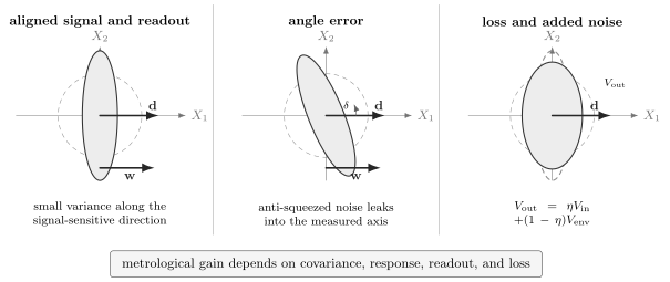
Squeezing improves a mean-shift estimate when the low-noise direction is matched to the response and readout. Angle error admixes the anti-squeezed variance; loss mixes the state with reference or environmental noise and rounds the covariance ellipse.

Angle Error and Anti-Squeezed Leakage

Let the principal normalized variances be $v_-=e^{-2r}$ and $v_+=e^{2r}$. If the readout is misaligned from the squeezed axis by an angle $\delta$, the measured variance is

$$v(\delta) = v_-\cos^2\delta + v_+\sin^2\delta.$$

For a random zero-mean angle error with small variance $\sigma_\delta^2$,

$$\mathbb E[v] \simeq v_- + (v_+-v_-) \sigma_\delta^2.$$

Stronger source squeezing therefore raises the phase-control requirement: the anti-squeezed variance grows exponentially and can dominate even through a small angular leak. “More squeezing” is not monotonic improvement when the readout phase is noisy.

The same geometry appears for collective spins. A fluctuating rotation axis, local-oscillator phase, or nonlinear readout maps anti-squeezed fluctuations into the estimator. Covariance must be propagated through the actual control sequence, not attached to a nominal axis at state-preparation time.

Optical Quadrature Example

For one bosonic mode, use

$$X = \frac{a+a^\dagger}{\sqrt2}, \qquad P = \frac{a-a^\dagger}{i\sqrt2}, \qquad [X,P]=i.$$

The vacuum variances are $1/2$. In one phase convention, an ideal squeezed vacuum has

$$(\Delta X)^2 = \frac12e^{-2r}, \qquad (\Delta P)^2 = \frac12e^{2r}.$$

For a bright field with real displacement $\alpha$ and a small phase shift $\phi$, suppose the mean phase-quadrature response is

$$\partial_\phi\langle P\rangle \simeq \sqrt2\,|\alpha|.$$

Phase-quadrature squeezing then gives

$$\Delta\phi \simeq \frac{e^{-r}}{2|\alpha|} = \frac{e^{-r}}{2\sqrt{n_{\mathrm c}}},$$

where $n_{\mathrm c}=|\alpha|^2$ is the coherent displacement energy in this simple model. The formula is local and assumes ideal alignment and readout. It does not charge the squeezed-vacuum energy

$$n_{\mathrm s} = \sinh^2r,$$

source pump, loss, or phase reference.

The optical canonical page develops what the mode is, how the state is generated, how homodyne spectra are normalized, and how source and observed squeezing differ. The metrological lesson here is narrower: reduced quadrature noise must be divided by the measured signal slope and compared under total-resource accounting.

Collective-Spin Preview

For $N$ effective spin-$1/2$ probes, define

$$J_k = \frac12 \sum_{j=1}^{N} \sigma_k^{(j)}.$$

A coherent spin state polarized along $x$ has

$$|\langle\mathbf J\rangle| = \frac N2, \qquad (\Delta J_y)^2 = (\Delta J_z)^2 = \frac N4.$$

The Kitagawa–Ueda noise-squeezing parameter is

$$\xi_S^2 = \frac{ 4\min_{\perp}(\Delta J_\perp)^2 }{N}.$$

It compares the narrowest transverse spin variance with coherent-spin noise. The Wineland metrological parameter includes the response or contrast:

$$\xi_R^2 = \frac{ N\min_{\perp}(\Delta J_\perp)^2 }{ |\langle\mathbf J\rangle|^2 }.$$

For a suitable small-angle Ramsey readout,

$$(\Delta\phi)^2 = \frac{\xi_R^2}{N}.$$

It is possible to have $\xi_S^2<1$ but little useful mean spin, so $\xi_R^2$ is the relevant local spectroscopic metric. Under the usual identical-particle collective-spin assumptions, $\xi_R^2<1$ also certifies multipartite entanglement. The converse fails: many entangled states are not spin-squeezed by this criterion, and some have metrological value requiring a nonlinear measurement.

One-axis twisting, two-axis countertwisting, collisional dynamics, cavity feedback, and quantum-nondemolition measurement can generate collective-spin squeezing. Their detailed scaling, entanglement depth, curvature, phase range, and clock implementation require a dedicated treatment; the formulas above serve only to distinguish variance squeezing from response-aware gain.

Differential and Multimode Squeezing

Squeezing need not reduce the marginal variance of one subsystem. For two readouts $X_A$ and $X_B$,

$$\operatorname{Var}(X_A-X_B) = \operatorname{Var}(X_A) + \operatorname{Var}(X_B) - 2\operatorname{Cov}(X_A,X_B).$$

Positive correlations can make the difference quieter than either marginal. This structure underlies twin-beam intensity-difference squeezing, EPR-like quadratures, differential clock comparisons, and distributed sensing.

The reference must follow the same mode transformation. Comparing a joint observable with the single-mode vacuum variance gives the wrong normalization. Likewise, common-mode technical-noise rejection can produce a quiet difference channel without nonclassical squeezing. A nonclassical or entanglement claim needs the appropriate separability or classical-state bound, not merely a low measured variance.

Loss, Thermal Noise, and Efficiency

Normalize a quadrature variance so that vacuum is one. A pure-loss channel of efficiency $\eta$ gives

$$v_{\mathrm{out}} = \eta v_{\mathrm{in}} + (1-\eta).$$

Even infinite input squeezing has the detector-plane floor

$$v_{\mathrm{out}} \ge 1-\eta.$$

If the environment has mean thermal occupation $n_{\mathrm{th}}$, the same attenuator model becomes

$$v_{\mathrm{out}} = \eta v_{\mathrm{in}} + (1-\eta) (2n_{\mathrm{th}}+1).$$

More explicitly, when environmental quadrature variance is normalized as $v_{\mathrm{env}}=2n_{\mathrm{th}}+1$,

$$v_{\mathrm{out}} = \eta v_{\mathrm{in}} + (1-\eta)v_{\mathrm{env}}.$$

The second form prevents a common bookkeeping error: the added thermal term is weighted by the lost fraction. In optical systems at ordinary carrier frequencies, the environmental mode is often close to vacuum; in microwave and mechanical systems, thermal occupancy can dominate.

Efficiency should include every unobserved mixing channel relevant to the mode: source escape, propagation, mode overlap, detector quantum efficiency, unmonitored atomic loss, and readout transfer. A single fitted $\eta$ may be a useful effective model, but it should not be mistaken for a diagnosis of which component caused the degradation.

Conditional and Unconditional Squeezing

A quantum-nondemolition or weak measurement can reduce the conditional variance of a collective variable given a measurement record $R$:

$$\operatorname{Var}(M\mid R) < \operatorname{Var}(M).$$

This is operationally useful if the record is retained and used for feedback, feed-forward, or the final estimator. If the record is discarded, the unconditional state can remain broad because different conditional means are mixed together.

The distinction is analogous to heralding. A low conditional variance does not define the per-attempt gain unless success probability, rejected trials, latency, and record acquisition are included. A complete report states whether squeezing is conditional, deterministic after feedback, or inferred only after retrospective subtraction.

Measurement-based squeezing also spends information. Reusing the same record to certify preparation and estimate the unknown parameter can create correlations that invalidate a naive independent-noise calculation. The full joint likelihood should include preparation and sensing records.

Squeezing and Fisher Information

For a one-dimensional Gaussian readout with parameter-dependent mean and fixed variance,

$$F_C = \frac{ (\partial_\theta\langle M\rangle)^2 }{ (\Delta M)^2 }.$$

The error-propagation variance is exactly $1/F_C$ in this local model. Squeezing improves the implemented Fisher information when it reduces the denominator without sacrificing the numerator.

The quantum Fisher information optimizes over all allowed measurements. A squeezed quadrature can make a simple homodyne, population, or linear detector nearly optimal, but variance squeezing is neither necessary nor sufficient for maximizing QFI. Non-Gaussian states may carry information in higher moments; a squeezed state measured on the wrong axis may leave most of its QFI inaccessible.

For collective spins generated by a linear rotation, $F_Q>N$ certifies entanglement and sub-SQL potential, while $\xi_R^2<1$ certifies that a specific mean-spin readout can realize such a gain. The QFI criterion is broader; the squeezing criterion is more tied to an operationally simple measurement.

Constant Gain Versus Scaling Gain

If a bright probe has $n_{\mathrm c}\propto N$ and the squeezing strength $r$ is held fixed, then

$$\Delta\theta \propto \frac{e^{-r}}{\sqrt N}.$$

The sensor has a constant sub-SQL factor but retains the $N^{-1/2}$ exponent. This can be extremely valuable: $10\ \mathrm{dB}$ of realized variance gain ideally replaces a factor of ten in averaging resource. It is not Heisenberg scaling.

To make the same local formula behave as $1/N$, one would need

$$e^{-r} \propto N^{-1/2},$$

so $r$ grows logarithmically. But then

$$n_{\mathrm s} = \sinh^2r \sim \frac N4$$

for large $r$ under this scaling. The squeezed field itself carries an extensive resource and becomes increasingly vulnerable to loss and phase error. A claim based only on the bright displacement $n_{\mathrm c}$ omits that cost.

Optimized lossless interferometers can use coherent displacement and squeezed vacuum together to approach inverse-total-energy scaling. Any such statement must specify total photons, phase reference, estimator range, and whether preparation or rejected events are charged. Under fixed nonzero loss, the asymptotic gain is generally bounded to a constant for standard independent loss models.

An End-to-End Squeezing Audit

Item	Question
estimand	Which phase, displacement, frequency, field, or derived quantity is inferred?
squeezed observable	Which operator or filtered data mode has reduced variance?
reference	What state or strategy sets the unsqueezed noise level?
response	What is $\partial_\theta\langle M\rangle$, including contrast and transfer functions?
resources	Are probe number, squeezed energy, time, pump, passes, bandwidth, and failed trials matched?
covariance	Are angle, cross-quadrature, temporal, and common-mode correlations retained?
loss and noise	Is the quoted value source-level, detector-level, or estimator-level?
inference	Are bias, phase wraps, conditioning records, and uncertainty coverage handled?
evidence	Are raw and corrected noise, anti-squeezing, calibration uncertainty, and task gain reported?

The strongest operational statement is not “the source produced $S$ dB.” It is “the complete sensor reduced a declared estimation risk by a measured factor under a matched resource boundary,” with the source squeezing and loss model supplied as supporting evidence.

Common Mistakes

Omitting the reference

“Reduced noise” has no meaning without a comparator in the same units and mode. An electronics floor or a noisy historical baseline is not necessarily a quantum-noise reference.

Reporting noise without response

A narrow distribution can be insensitive to the parameter. Divide by the calibrated slope or use the full likelihood.

Ignoring anti-squeezing

Angle jitter, detuning, nonlinear evolution, and imperfect control can rotate the broad quadrature into the readout.

Calling squeezing entanglement

Single-mode squeezing is nonclassical under an optical coherent-state criterion but is not bipartite entanglement until a subsystem split is specified. Spin-squeezing entanglement witnesses require their stated particle and symmetry assumptions.

Confusing source and observed decibels

Loss-corrected source inference and directly observed detector-plane noise are different quantities. The final estimator may see still another gain.

Treating fixed squeezing as a new exponent

A constant $e^{-r}$ improves the prefactor of $N^{-1/2}$ scaling. It does not turn that law into $N^{-1}$.

Hiding conditioning cost

Postselection or a preparation record can make a conditional ensemble quiet. Failures, latency, and use of the record belong in the end-to-end protocol.

Using one covariance number for every frequency

Continuous sensors have mode- and frequency-dependent squeezing angle, variance, and loss. Integrate the noise against the signal waveform and estimator filter.

Exercises

1. Minimum-uncertainty redistribution

An ideal mode has variances

$$(\Delta X)^2 = \frac12e^{-2r}, \qquad (\Delta P)^2 = \frac12e^{2r}.$$

Verify the uncertainty product and find the variance squeezing in decibels for $r=0.5$.

Solution

The product of variances is

$$(\Delta X)^2(\Delta P)^2 = \frac14,$$

so $\Delta X\Delta P=1/2$. Relative to vacuum, the squeezed variance factor is $e^{-2r}=e^{-1}$. Its positive squeezing magnitude is

$$S_{\mathrm{dB}} = -10\log_{10}(e^{-1}) \approx 4.34\ \mathrm{dB}.$$

2. Optimal linear readout

For a Gaussian measurement vector with covariance $V\succ0$ and response $\mathbf d$, show that

$$\frac{(\mathbf w^{\mathsf T}\mathbf d)^2} {\mathbf w^{\mathsf T}V\mathbf w} \le \mathbf d^{\mathsf T}V^{-1}\mathbf d.$$

Solution

Write

$$\mathbf w^{\mathsf T}\mathbf d = (V^{1/2}\mathbf w)^{\mathsf T} (V^{-1/2}\mathbf d).$$

Cauchy–Schwarz gives

$$(\mathbf w^{\mathsf T}\mathbf d)^2 \le (\mathbf w^{\mathsf T}V\mathbf w) (\mathbf d^{\mathsf T}V^{-1}\mathbf d).$$

Dividing by the positive readout variance proves the bound. Equality requires $V^{1/2}\mathbf w\propto V^{-1/2}\mathbf d$, or $\mathbf w\propto V^{-1}\mathbf d$.

3. Angle leakage

A state has $10\ \mathrm{dB}$ squeezing and $15\ \mathrm{dB}$ anti-squeezing in variance. Find the measured normalized variance at a fixed angle error $\delta=3^\circ$.

Solution

The principal variances are

$$v_- = 10^{-10/10} = 0.1, \qquad v_+ = 10^{15/10} \approx 31.62.$$

Therefore

$$\begin{aligned} v(3^\circ) &= 0.1\cos^2(3^\circ) +31.62\sin^2(3^\circ) \\ &\approx 0.186. \end{aligned}$$

The observed squeezing is

$$-10\log_{10}(0.186) \approx 7.30\ \mathrm{dB}.$$

A small angle error has discarded about $2.7\ \mathrm{dB}$ because the anti-squeezed variance is large.

4. Loss ceiling

An input has normalized variance $v_{\mathrm{in}}=0.10$ and total efficiency $\eta=0.80$. Find the output variance and observed squeezing. What is the best possible observed squeezing at that efficiency?

Solution

Pure loss gives

$$v_{\mathrm{out}} = 0.80(0.10)+0.20 = 0.28.$$

Thus

$$S_{\mathrm{obs}} = -10\log_{10}(0.28) \approx 5.53\ \mathrm{dB}.$$

As $v_{\mathrm{in}}\to0$, the output approaches $1-\eta=0.20$, corresponding to a ceiling of

$$-10\log_{10}(0.20) \approx 6.99\ \mathrm{dB}.$$

5. Noise squeezing versus metrological squeezing

A preparation reduces readout variance to $0.40$ of the reference but also reduces the signal slope to $0.60$ of the reference. Compute $\xi_{\mathrm{met}}^2$.

Solution

The error-propagation variance ratio is

$$\xi_{\mathrm{met}}^2 = \frac{0.40}{0.60^2} \approx 1.11.$$

Although the observable is noise-squeezed, the parameter estimate is about $11\%$ worse in variance because the response loss is larger.

6. Spin contrast penalty

An $N$-atom state has minimum transverse variance $(\Delta J_\perp)^2=0.10N$ and mean-spin length $|\langle\mathbf J\rangle|=0.30N$. Find $\xi_S^2$ and $\xi_R^2$. Is the state metrologically squeezed by the Wineland criterion?

Solution

The noise parameter is

$$\xi_S^2 = \frac{4(0.10N)}{N} = 0.40.$$

The response-aware parameter is

$$\xi_R^2 = \frac{N(0.10N)}{(0.30N)^2} = \frac{0.10}{0.09} \approx 1.11.$$

The transverse variance is squeezed, but the reduced mean-spin contrast removes the local spectroscopic gain.

7. Correlation-squeezed difference

Two readouts have equal variance $V$ and covariance $cV$. Find the variance of $X_A-X_B$. For what $c$ is the difference variance below the independent reference $2V$?

Solution

Using the covariance identity,

$$\operatorname{Var}(X_A-X_B) = 2V-2cV = 2V(1-c).$$

It is below $2V$ whenever $c>0$. This establishes a quieter difference channel, not by itself nonclassicality or entanglement; a classical common fluctuation can also produce positive covariance.

8. Audit a squeezing claim

An experiment reports “$8\ \mathrm{dB}$ metrological squeezing” after subtracting detector noise and selecting $25\%$ of trials. List the minimum additional information needed to interpret the claim.

Solution

The report should identify the squeezed observable and reference; give raw detector-plane noise and the subtraction model; report anti-squeezing, efficiency, phase stability, and calibration uncertainty; measure the signal slope or Fisher information; include all attempted probes and elapsed time; state the selection criterion and whether failures carry information; compare against a resource-matched unsqueezed strategy; and validate estimator bias, uncertainty coverage, and task-level gain. Without these items, the number could describe source inference or conditional noise rather than end-to-end metrological improvement.

References

1. H. P. Robertson, “The uncertainty principle,” Physical Review 34, 163–164 (1929), doi:10.1103/PhysRev.34.163.
2. E. Schrödinger, “Zum Heisenbergschen Unschärfeprinzip,” Sitzungsberichte der Preussischen Akademie der Wissenschaften, Physikalisch-mathematische Klasse 14, 296–303 (1930), English translation.
3. H. P. Yuen, “Two-photon coherent states of the radiation field,” Physical Review A 13, 2226–2243 (1976), doi:10.1103/PhysRevA.13.2226.
4. D. F. Walls, “Squeezed states of light,” Nature 306, 141–146 (1983), doi:10.1038/306141a0.
5. C. M. Caves, “Quantum-mechanical noise in an interferometer,” Physical Review D 23, 1693–1708 (1981), doi:10.1103/PhysRevD.23.1693.
6. R. E. Slusher, L. W. Hollberg, B. Yurke, J. C. Mertz, and J. F. Valley, “Observation of squeezed states generated by four-wave mixing in an optical cavity,” Physical Review Letters 55, 2409–2412 (1985), doi:10.1103/PhysRevLett.55.2409.
7. L.-A. Wu, H. J. Kimble, J. L. Hall, and H. Wu, “Generation of squeezed states by parametric down conversion,” Physical Review Letters 57, 2520–2523 (1986), doi:10.1103/PhysRevLett.57.2520.
8. D. J. Wineland, J. J. Bollinger, W. M. Itano, F. L. Moore, and D. J. Heinzen, “Spin squeezing and reduced quantum noise in spectroscopy,” Physical Review A 46, R6797–R6800 (1992), doi:10.1103/PhysRevA.46.R6797.
9. M. Kitagawa and M. Ueda, “Squeezed spin states,” Physical Review A 47, 5138–5143 (1993), doi:10.1103/PhysRevA.47.5138.
10. A. Sørensen, L.-M. Duan, J. I. Cirac, and P. Zoller, “Many-particle entanglement with Bose–Einstein condensates,” Nature 409, 63–66 (2001), doi:10.1038/35051038.
11. J. Ma, X. Wang, C. P. Sun, and F. Nori, “Quantum spin squeezing,” Physics Reports 509, 89–165 (2011), doi:10.1016/j.physrep.2011.08.003.
12. L. Pezzè, A. Smerzi, M. K. Oberthaler, R. Schmied, and P. Treutlein, “Quantum metrology with nonclassical states of atomic ensembles,” Reviews of Modern Physics 90, 035005 (2018), doi:10.1103/RevModPhys.90.035005.
13. S. L. Braunstein and P. van Loock, “Quantum information with continuous variables,” Reviews of Modern Physics 77, 513–577 (2005), doi:10.1103/RevModPhys.77.513.
14. C. Weedbrook et al., “Gaussian quantum information,” Reviews of Modern Physics 84, 621–669 (2012), doi:10.1103/RevModPhys.84.621.
15. O. Pinel, P. Jian, N. Treps, C. Fabre, and D. Braun, “Quantum parameter estimation using general single-mode Gaussian states,” Physical Review A 88, 040102(R) (2013), doi:10.1103/PhysRevA.88.040102.
16. M. G. A. Paris, “Quantum estimation for quantum technology,” International Journal of Quantum Information 7, 125–137 (2009), doi:10.1142/S0219749909004839.
17. H. Vahlbruch, M. Mehmet, K. Danzmann, and R. Schnabel, “Detection of 15 dB squeezed states of light and their application for the absolute calibration of photoelectric quantum efficiency,” Physical Review Letters 117, 110801 (2016), doi:10.1103/PhysRevLett.117.110801.
18. J. Aasi et al. (LIGO Scientific Collaboration), “Enhanced sensitivity of the LIGO gravitational wave detector by using squeezed states of light,” Nature Photonics 7, 613–619 (2013), doi:10.1038/nphoton.2013.177.
19. F. Acernese et al. (Virgo Collaboration), “Increasing the astrophysical reach of the Advanced Virgo detector via the application of squeezed vacuum states of light,” Physical Review Letters 123, 231108 (2019), doi:10.1103/PhysRevLett.123.231108.
20. O. Hosten, N. J. Engelsen, R. Krishnakumar, and M. A. Kasevich, “Measurement noise 100 times lower than the quantum-projection limit using entangled atoms,” Nature 529, 505–508 (2016), doi:10.1038/nature16176.
21. I. D. Leroux, M. H. Schleier-Smith, and V. Vuletić, “Implementation of cavity squeezing of a collective atomic spin,” Physical Review Letters 104, 073602 (2010), doi:10.1103/PhysRevLett.104.073602.
22. M. H. Schleier-Smith, I. D. Leroux, and V. Vuletić, “States of an ensemble of two-level atoms with reduced quantum uncertainty,” Physical Review Letters 104, 073604 (2010), doi:10.1103/PhysRevLett.104.073604.
23. K. C. Cox, G. P. Greve, J. M. Weiner, and J. K. Thompson, “Deterministic squeezed states with collective measurements and feedback,” Physical Review Letters 116, 093602 (2016), doi:10.1103/PhysRevLett.116.093602.
24. G. Tóth and I. Apellaniz, “Quantum metrology from a quantum information science perspective,” Journal of Physics A 47, 424006 (2014), doi:10.1088/1751-8113/47/42/424006.

Further Connections

• Quantum Measurement as Estimation supplies the estimand, likelihood, estimator, loss, uncertainty, and validation contract.
• Classical and Quantum Fisher Information connects implemented readout noise to Fisher information and broader measurement optimization.
• Standard Quantum Limit defines the independent-probe reference that a sub-SQL squeezing claim must match.
• Heisenberg Scaling distinguishes fixed squeezing gain from an inverse-resource asymptotic law.
• Spin Squeezing specializes the covariance-and-response framework to collective spins, Ramsey readout, entanglement certification, and clocks.
• Squeezed Light develops optical preparation, mode definitions, sideband spectra, homodyne detection, loss inference, and interferometer injection.
• Mach–Zehnder Interferometry places squeezed-input gains inside a complete optical phase-reference, loss, resource, and comparator audit.
• Squeezed States as Entangled Modes develops two-mode squeezing, Schmidt structure, and EPR-like correlations.
• Sensing Case Studies examines realized clock and interferometer gains under end-to-end resource accounting.
• Precision Measurement and Metrology connects squeezing to clocks, force sensing, field measurements, and complete instrument budgets.