NV-Center Sensing

A negatively charged nitrogen-vacancy center, NV$^-$, combines an electronic spin, optical initialization and fluorescence readout, microwave control, and atomic-scale localization in diamond. Those ingredients make it a versatile transducer, but they do not define one universal sensor. Continuous-wave ODMR, Ramsey magnetometry, echo and dynamical-decoupling spectroscopy, and $T_1$ relaxometry generate different data and estimate different properties of the environment.

This page is the canonical home for end-to-end NV-center sensing as a quantum-estimation case study. It connects the photon record to a likelihood, chooses protocols by estimand, derives comparison-ready sensitivity measures, and treats depth, standoff, orientation, field inversion, nuisance rejection, sample disturbance, and validation as parts of the measurement.

NV Centers and Solid-State Defects owns the ground-state model, optical pumping, fluorescence backaction, charge dynamics, relaxation, dephasing, and the extension to other defects. Defect and Solid-State Spin Qubits owns materials, fabrication, spin registers, photonic interfaces, networking, and architecture-level hardware evidence. Magnetometry owns the platform-neutral theory of spatiotemporal field modes, Fisher information, bandwidth, vector incompatibility, and resource matching. The Sensing Case Studies page owns the historical evidence narrative, including the corrected ensemble sensitivity claim discussed there.

The Sensing Contract

An NV experiment should be specified by a tuple such as

$$\mathcal S_{mathrm{NV}} = (\theta,\rho_{\mathrm{NV}},\mathcal C, \mathcal M,\mathcal G,\mathcal E).$$

Here

• $\theta$ is the estimand: a field component, waveform amplitude, noise spectrum, temperature, source parameter, or image;
• $\rho_{\mathrm{NV}}$ is the prepared spin and charge-state ensemble;
• $\mathcal C$ is the optical and microwave control sequence;
• $\mathcal M$ is the photon-count or camera likelihood;
• $\mathcal G$ is the spatial geometry, including depth and standoff; and
• $\mathcal E$ is the estimator, calibration model, and uncertainty statement.

Changing any element can change the meaning of the result. For example, a shallow single NV under an XY8 sequence can estimate an AC magnetic-noise mode from a nanoscale sample. A thick NV ensemble under continuous-wave excitation can estimate a slowly varying field projection in each camera pixel. The former emphasizes proximity and spectral selectivity; the latter emphasizes parallelism and photon rate.

Minimal Spin Model and Frequency Conventions

Using dimensionless spin-1 operators, a common effective ground-state model is

$$\frac{H}{\hbar} = D S_z^2 + \gamma_e\mathbf B\cdot\mathbf S + E(S_x^2-S_y^2) + H_{\mathrm{hf}} + H_{\mathrm{other}}.$$

The NV axis defines $z$, $D/(2\pi)$ is approximately $2.87\,\mathrm{GHz}$ near room temperature, and

$$\frac{|\gamma_e|}{2\pi} \simeq 28.0\,\mathrm{GHz/T}.$$

The precise values, signs, and environmental shifts belong in the calibration. Near an axial bias field large enough to resolve the two branches,

$$\nu_\pm \simeq \frac{D+\delta_{\mathrm{cm}}}{2\pi} \pm \frac{|\gamma_e|}{2\pi}B_\parallel.$$

The term $\delta_{\mathrm{cm}}$ collects common-mode shifts from temperature, longitudinal strain, and other perturbations at the chosen operating point. The branch average and difference are therefore approximately

$$\begin{aligned} \frac{\nu_++\nu_-}{2} &\simeq \frac{D+\delta_{\mathrm{cm}}}{2\pi}, \\ \nu_+-\nu_- &\simeq 2\frac{|\gamma_e|}{2\pi}B_\parallel. \end{aligned}$$

This common-versus-differential structure is central to nuisance rejection. It is only approximate when transverse fields, strain mixing, hyperfine structure, or level anticrossings matter. Fitting the simple linear formula outside that regime biases the inferred field.

Diamond supplies four crystallographic NV orientation classes. A single resolved class measures one projection $\mathbf n_i\cdot\mathbf B$; it does not directly measure the full vector field.

Fluorescence Is a Likelihood, Not a Spin Value

Off-resonant optical excitation usually prepares population preferentially in $m_s=0$ and produces spin-dependent fluorescence during readout. Let $q_0(\theta)$ be the probability that the final spin is in the bright state. A simple single-shot photon model is a mixture of Poisson distributions:

$$p(n\mid\theta) = q_0(\theta) e^{-\alpha_0}\frac{\alpha_0^n}{n!} + [1-q_0(\theta)] e^{-\alpha_1}\frac{\alpha_1^n}{n!},$$

where $\alpha_0>\alpha_1$ are the mean detected counts conditioned on the two spin classes. Optical pumping during readout, background fluorescence, charge-state conversion, detector dead time, and time gating can require a richer model.

The classical Fisher information in the photon record is

$$F_\theta = \sum_{n=0}^{\infty} \frac{ [\partial_\theta p(n\mid\theta)]^2 }{p(n\mid\theta)}.$$

This expression automatically penalizes poor photon collection and overlapping bright and dark distributions. Replacing fluorescence with an ideal projective spin measurement can overstate the available information by orders of magnitude, especially for room-temperature single-shot readout.

Reference windows are often used to normalize laser intensity and fluorescence drift. They add data but also consume time and can introduce covariance. The likelihood should include signal and reference counts jointly rather than treating the normalized ratio as noiseless.

For a cycle of duration $T_c$ with per-cycle information $F_\theta^{(1)}$, the local information rate is

$$\dot F_\theta = \frac{F_\theta^{(1)}}{T_c}.$$

This is the cleanest bridge from a spin protocol to a comparison-ready sensor metric.

Continuous-Wave ODMR

In continuous-wave optically detected magnetic resonance (CW ODMR), optical and microwave drives are applied together while fluorescence is recorded as a function of microwave frequency. A simple isolated resonance is

$$R(\nu;B) = R_0 \left[ 1-C_{\mathrm{ODMR}} L(\nu-\nu_0(B)) \right] +R_{\mathrm{bg}},$$

with Lorentzian

$$L(x) = \frac{1}{1+4x^2/(\Delta\nu)^2}.$$

Here $\Delta\nu$ is the full width at half maximum and $C_{\mathrm{ODMR}}$ is the fractional contrast. For Poisson counts collected for time $t$ at one working frequency,

$$F_B = t \frac{[\partial_B R(\nu;B)]^2}{R(\nu;B)}.$$

The input-referred photon-shot-noise floor is therefore

$$\eta_B(\nu) = \frac{\sqrt{R(\nu;B)}} {|\partial_B R(\nu;B)|}.$$

For an isolated low-contrast Lorentzian, negligible background, and frequency gyromagnetic ratio $g_e=|\gamma_e|/(2\pi)$, optimizing the slope gives

$$\eta_B^{\mathrm{CW}} \simeq \frac{4}{3\sqrt3} \frac{\Delta\nu} {C_{\mathrm{ODMR}}g_e\sqrt{R_0}}.$$

This useful expression is not universal. Power broadening changes $\Delta\nu$, optical and microwave powers change contrast and photon rate, neighboring hyperfine and orientation lines distort the slope, and technical laser noise violates the Poisson model. Frequency modulation and lock-in detection can reject slow intensity drift, but the measured complex transfer function and demodulation bandwidth still need calibration.

CW ODMR is operationally simple and naturally supports imaging. It is often a good choice when moderate DC bandwidth, robust acquisition, or many camera pixels matter more than maximum per-spin information. A full spectrum is also valuable for identifying branches and nuisance structure before operating a locked sensor.

Pulsed Phase Sensing

A pulsed experiment separates initialization, coherent evolution, and readout. For a selected two-level subspace, the accumulated magnetic phase is

$$\phi_B = \gamma_e \int_0^T y(t)B_\parallel(t)\,dt.$$

If the final bright-state probability is

$$q_0(B) = \frac12 \left[ 1+C_s\sin(\phi_B+\vartheta) \right],$$

then the spin-state contrast $C_s$ describes coherent preparation and evolution. The photon likelihood adds a separate readout penalty through $\alpha_0$ and $\alpha_1$. Conflating those two contrasts hides where information was lost.

An effective fringe contrast $C_{\mathrm{eff}}$ can be used for a compact benchmark when its calibration is stated. For $N_{\mathrm{eff}}$ independent, equivalently coupled NV centers,

$$\eta_B \simeq \frac{\sqrt{T_c}} {C_{\mathrm{eff}}|\gamma_e|\, |\mathcal A|\sqrt{N_{\mathrm{eff}}}}, \qquad \mathcal A = \int_0^T y(t)s(t)\,dt.$$

For actual analysis, evaluating the Fisher information of the measured photon likelihood is preferable to assigning one catch-all contrast.

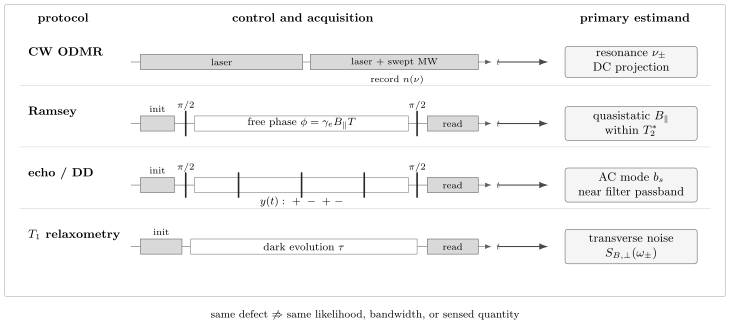
Four protocols interrogate different properties of the same defect. CW ODMR tracks a resonance, Ramsey measures quasistatic phase, echo or dynamical decoupling selects an AC temporal mode, and $T_1$ relaxometry probes transverse noise near a spin-transition frequency. Their sensitivities are not interchangeable.

Ramsey sensing

For Ramsey sensing, $y(t)=1$ during free evolution. It responds to a static or slowly varying field over a time usually limited by $T_2^*$. The local phase slope grows as $T$, while dephasing and phase aliases constrain useful interrogation. The result is a projection along the selected NV axis at the chosen bias point.

Double-quantum coherence

A double-quantum (DQ) protocol prepares coherence between $m_s=+1$ and $m_s=-1$. Its magnetic phase is approximately

$$\phi_{\mathrm{DQ}} = 2\gamma_e \int_0^T y(t)B_\parallel(t)\,dt.$$

The factor of two increases phase slope, while shifts common to both $m_s=\pm1$ levels cancel to first order. DQ sensing can therefore reject temperature and longitudinal-strain shifts that broaden single-quantum ensembles. It is not automatically twice as sensitive: preparation and readout errors, microwave inhomogeneity, altered coherence, and overhead must be included. Transverse mixing and imperfect branch symmetry can leave residual nuisance response.

Echo and dynamical decoupling

Hahn echo and multipulse sequences change the sign of $y(t)$. They suppress slow sensor-frequency noise while retaining target fields whose sign matches the toggling pattern. A sequence with interpulse spacing $\tau$ has response near frequencies of order $1/(2\tau)$, with convention-dependent harmonics and finite-pulse corrections.

The same filter acts on target and environmental fields. A narrow coherence dip may indicate a coherent signal, a stochastic spectral feature, a nearby nuclear spin, a pulse harmonic, or control error. Phase cycling, sequence variation, field dependence, and independent calibration are needed to distinguish them. Dynamical Decoupling develops the filter functions in detail.

Correlation and synchronized spectroscopy

One coherent evolution interval need not set the ultimate spectral resolution. Correlation spectroscopy and clock-referenced repeated measurements encode the signal phase across separated windows. Resolution can then be set by the total record length or reference-clock stability, while sensitivity still depends on per-window coherence, readout, dead time, and signal phase memory. Long Fourier records do not evade those resource costs.

Longitudinal Relaxometry

$T_1$ relaxometry asks a different question. Prepare a spin population, wait in the dark for time $\tau$, and read out the survival probability. A simple fit model is

$$P_0(\tau) = P_\infty + [P_0(0)-P_\infty]e^{-\Gamma_1\tau},$$

although the spin-1 level structure can require multiple rates. Additional transverse magnetic noise contributes schematically

$$\Gamma_1^{\mathrm{ext}} \propto \gamma_e^2 S_{B,\perp}(\omega_\pm),$$

with tensor projections and one-sided or two-sided factors fixed by the spectral convention. Sweeping the bias field tunes $\omega_\pm$ and samples different parts of the environmental spectrum.

Relaxometry detects fluctuations that exchange energy with the NV spin. It can probe paramagnetic molecules, Johnson noise, spin waves, and magnetic phase dynamics even when the mean stray field vanishes. It does not directly return a deterministic DC field, and a measured change in $T_1$ is not itself a noise PSD until a coupling geometry and rate model are supplied.

Optimizing the dark time requires the full count likelihood. Waiting much longer than $T_1$ produces equilibrium populations with little rate information; waiting too briefly produces little contrast. Background relaxation should be measured at matched temperature, depth, optical history, and bias field.

Spatial Transfer and Standoff

The atomic scale of an NV wavefunction does not by itself guarantee atomic spatial resolution. A magnetic dipole $\boldsymbol\mu$ at displacement $\mathbf r$ produces

$$\mathbf B_{\mathrm{dip}}(\mathbf r) = \frac{\mu_0}{4\pi r^3} \left[ 3(\boldsymbol\mu\cdot\widehat{\mathbf r}) \widehat{\mathbf r} - \boldsymbol\mu \right].$$

The signal can therefore change sharply with NV depth and tip-to-sample gap. If the distance doubles, a point-dipole field falls by a factor of eight. Uncertainty in depth can dominate the inferred moment or spin density.

For planar sources, a spatial Fourier component with lateral wave number $k$ typically reaches a sensor at height $d$ with a factor proportional to $e^{-kd}$. High-spatial-frequency structure is exponentially suppressed. Deconvolution can amplify those components, but it also amplifies noise and model error. A magnetic image should report the measured projection and height before presenting a source reconstruction.

Scanning single NV

A scanning probe places one shallow NV near a sample and records one field projection or noise statistic point by point. Its strengths are proximity, small sensing volume, and operation over wide temperature and field ranges. Its limitations include photon rate, scan time, tip wear, topographic cross-talk, uncertain NV position and axis, drift, and perturbation from the probe or applied microwaves.

Wide-field and confocal ensembles

An ensemble provides parallel pixels and more photons. The effective number of sensors in a pixel is not simply the implanted density times the nominal volume. Orientation selection, charge-state fraction, optical point-spread function, depth distribution, microwave field, collection efficiency, and analysis weighting all matter.

Increasing density can shorten $T_2^*$ through paramagnetic impurities, dipolar interactions, strain inhomogeneity, and charge instability. Camera binning improves count statistics while reducing spatial resolution and introducing correlated noise through optics and image processing. Sensitivity per pixel should always be paired with pixel area, NV-layer thickness, standoff, and measured point-spread response.

Vector Reconstruction from Four Orientations

Choose directed unit vectors $\mathbf n_i$ along the four tetrahedral NV axes. In the ideal geometry,

$$\sum_{i=1}^{4}\mathbf n_i=0, \qquad \sum_{i=1}^{4} \mathbf n_i\mathbf n_i^{\mathsf T} = \frac43 I.$$

If spectroscopy identifies the signed projections $b_i=\mathbf n_i\cdot\mathbf B$, then

$$\mathbf B = \frac34 \sum_{i=1}^{4}b_i\mathbf n_i.$$

Real reconstruction is a weighted inverse problem. Resonance overlap, orientation-dependent contrast, unequal linewidths, strain, hyperfine structure, bias-field uncertainty, and camera-pixel covariance should enter a design matrix and covariance model. If only transition splittings are known, sign ambiguities may remain unless a bias field or branch assignment resolves them.

The four-orientation formula estimates the local vector field at the NV layer. Inferring current density, magnetization, or spin texture from that field is a second inverse problem with boundary conditions and regularization. Maxwell constraints can help, but they do not make an underdetermined source unique.

Nanoscale Nuclear Magnetic Resonance

Near-surface NV centers can detect nuclear-spin fields from volumes far smaller than conventional inductive NMR. At that scale, statistical polarization can exceed the mean thermal polarization. The observed quantity is then often a field variance or correlation rather than a phase-coherent mean field:

$$\langle B(t)\rangle \simeq0, \qquad \langle B(t)B(0)\rangle \ne0.$$

For a spin density $\rho$ above a shallow NV, dipolar coupling gives the rough scaling

$$B_{\mathrm{rms}}^2 \propto \rho \int d^3r\,r^{-6} \propto \frac{\rho}{d^3},$$

up to angular factors and sample geometry. Thus $B_{\mathrm{rms}}\propto\sqrt\rho\,d^{-3/2}$ in the ideal half-space model. The depth inferred from a proton layer is model-dependent; surface roughness, adsorbates, finite thickness, diffusion, and pulse errors can shift it.

An XY8 or related sequence can reveal a response near a nuclear Larmor frequency. Establishing chemical identity or molecular structure requires more than matching one dip frequency. Field scaling, isotope controls, harmonic checks, correlation times, spectral resolution, surface chemistry, and a quantitative coupling model are needed. Diffusion can broaden nanoscale liquid signals because molecules move through a strongly inhomogeneous near-field kernel.

Detection of an ensemble’s statistical polarization should not be described as single-nucleus detection. Conversely, a coherently coupled individual nuclear spin in the diamond host is a different regime from external ensemble NMR.

Magnetic and Nonmagnetic Nuisance Responses

NV centers respond to several environmental variables. That versatility is a feature when the variable is the target and a cross-sensitivity when it is not.

Temperature, strain, and electric fields

Temperature changes $D$; strain and electric fields shift and mix levels. Branch differencing or DQ coherence rejects common-mode shifts to first order, while branch averaging can be used for thermometry. Neither operation removes all effects of transverse fields, line-shape changes, or spatially varying contrast. The response matrix should be calibrated over the actual operating range.

Charge and optical history

Optical power affects NV$^-$ population, NV$^0$ background, spin polarization, readout contrast, local heating, and sample photochemistry. A dark interval does not necessarily erase the preparation history. Laser-power references and charge-state diagnostics are especially important near surfaces and in nanodiamonds.

Microwave control

Microwave amplitude and detuning errors alter pulse area and filter functions. Conductors or magnetic samples can distort the near field, while microwave dissipation can heat the sample. A sequence that performs well on an isolated calibration NV may not have the same transfer function across an ensemble image.

Hyperfine and orientation structure

The host nitrogen and nearby $^{13}\mathrm C$ spins produce resolved or unresolved hyperfine features. They can serve as resources, spectral labels, or coherent ancillas, but ignoring them can bias resonance centers and create spurious filter responses. The chosen nuclear-spin state and polarization protocol belong in the measurement model.

Choosing a Protocol

Target	Natural starting protocol	Main response	Frequent limiting factors
Static or slowly varying field	CW ODMR or Ramsey	Resonance shift or free phase	Linewidth, $T_2^*$, drift, phase range
Known AC waveform	Echo or dynamical decoupling	Filtered coherent phase	$T_2$, pulse errors, timing, harmonics
Unknown narrowband coherent tone	Correlation or synchronized spectroscopy	Phase across repeated windows	Clock stability, dead time, phase memory
Magnetic noise near the NV transition	$T_1$ relaxometry	Population-relaxation rate	Background $T_1$, rate model, geometry
Nanoscale nuclear-spin fluctuations	Multipulse correlation spectroscopy	Coherence loss or correlation	Depth, diffusion, surface noise, aliases
Wide-field vector map	Multi-orientation ODMR	Several resonance projections	Line overlap, strain, pixel covariance

The table gives starting points, not exclusive assignments. Hybrid protocols can combine a coarse ODMR spectrum, a locked Ramsey channel, and intermittent calibration. The final choice should maximize information for the declared task per unit wall time, sample dose, and acceptable disturbance.

Worked CW Benchmark

Suppose an isolated Lorentzian has

$$\Delta\nu=1.0\,\mathrm{MHz}, \qquad C_{\mathrm{ODMR}}=0.030, \qquad R_0=5.0\times10^5\,\mathrm{s^{-1}}.$$

Using $g_e=28.0\,\mathrm{GHz/T}$ gives

$$\begin{aligned} \eta_B^{\mathrm{CW}} &\simeq \frac{4}{3\sqrt3} \frac{10^6} {0.030(28.0\times10^9) \sqrt{5.0\times10^5}} \\ &\simeq 1.3\times10^{-6} \ \mathrm{T}/\sqrt{\mathrm{Hz}}. \end{aligned}$$

This is a photon-shot-noise benchmark near the optimum slope. A measured spectrum can be worse because of laser noise, frequency drift, background, overlapping lines, and estimator inefficiency. A pulsed protocol may improve the result by separating optical broadening from coherent evolution, but only after preparation and readout overhead are counted.

Evidence and Reporting

A mature NV sensing report should make the full inference reproducible:

1. Sample: diamond growth, isotope content, NV and impurity densities, charge-state fraction, orientation populations, depth distribution, and surface treatment.
2. Geometry: NV axis, bias field, active volume or pixel, optical point spread, standoff, scan registration, and source model.
3. Protocol: optical wavelengths and powers, microwave waveform, pulse sequence, timing, phase cycle, duty factor, and rejected shots.
4. Likelihood: raw photon or camera counts, reference channels, background, detector model, and estimator.
5. Transfer: calibrated field amplitude and direction, complex frequency response, spatial kernel, dynamic range, and recovery.
6. Noise: raw and input-referred spectra, Allan-family diagnostics, covariance among pixels or repetitions, and visible noise subtraction.
7. Nuisances: temperature, strain, electric fields, charge conversion, optical heating, microwave heating, motion, and topography.
8. Comparison: matched NV number, volume, standoff, bandwidth, averaging time, sample dose, prior range, and classical reference.
9. Validation: blind injected signals, negative controls, sequence and bias-field reversals, synthetic-data recovery, and independent checks.
10. Provenance: calibration data, processing code, exclusions, uncertainty propagation, article corrections, and software versions.

State-level coherence, photon-shot-noise sensitivity, an input-referred sensor floor, a reconstructed source image, and a biological or materials conclusion are different evidence levels. A result can be strong at one level without yet establishing the next.

Common Mistakes

Calling every dip a magnetic resonance

Pulse harmonics, nuclear-spin aliases, microwave detuning, charge changes, and control errors can all produce features. Test field and sequence scaling.

Equating an atomic defect with atomic resolution

Depth, standoff, drift, point-spread response, and inverse-problem conditioning set the actual resolution.

Using ideal spin projection noise for fluorescence data

Room-temperature optical readout commonly collects few photons before spin information is erased. Use the photon likelihood or a measured readout-noise factor.

Quoting one sensitivity for every protocol

CW, Ramsey, DD, and relaxometry estimate different quantities over different bands. Preserve the estimand and transfer function with the number.

Assuming DQ removes every nuisance

DQ rejects common-mode shifts only to the accuracy of the spin Hamiltonian, control, and line model. Transverse mixing and line-shape variation remain.

Treating a coherence dip as a mean field

Nanoscale NMR often detects statistical polarization through variance or correlation. The mean can be zero.

Reconstructing a source without showing the measured field

Current or magnetization maps depend on height, boundary conditions, regularization, and priors. Publish the field projection and covariance too.

Ignoring sample disturbance

Laser and microwave heating, photoactivation, bias fields, and tip forces can change the system being measured. Disturbance is part of the resource ledger.

Exercises

1. Common and differential resonance shifts

Suppose

$$\nu_\pm = 2.870000\,\mathrm{GHz} +50\,\mathrm{kHz} \pm g_e B_\parallel,$$

with $g_e=28.0\,\mathrm{GHz/T}$, and the measured resonances are $\nu_+=2.871450\,\mathrm{GHz}$ and $\nu_-=2.868650\,\mathrm{GHz}$. Infer the common-mode shift and $B_\parallel$.

Solution

The average is

$$\frac{\nu_++\nu_-}{2} = 2.870050\,\mathrm{GHz},$$

so the common-mode shift from $2.870000\,\mathrm{GHz}$ is $50\,\mathrm{kHz}$. The splitting is

$$\nu_+-\nu_- = 2.800\,\mathrm{MHz}.$$

Therefore

$$B_\parallel = \frac{2.800\times10^6} {2(28.0\times10^9)} = 5.00\times10^{-5}\ \mathrm T = 50.0\ \mu\mathrm T.$$

2. CW photon-shot-noise floor

Use the Lorentzian benchmark to evaluate a resonance with $\Delta\nu=2.0\,\mathrm{MHz}$, $C_{\mathrm{ODMR}}=0.020$, and $R_0=2.0\times10^5\,\mathrm{s^{-1}}$. Take $g_e=28.0\,\mathrm{GHz/T}$.

Solution

Substitution gives

$$\eta_B^{\mathrm{CW}} = \frac{4}{3\sqrt3} \frac{2.0\times10^6} {0.020(28.0\times10^9) \sqrt{2.0\times10^5}}.$$

Numerically,

$$\eta_B^{\mathrm{CW}} \simeq 6.1\times10^{-6} \ \mathrm{T}/\sqrt{\mathrm{Hz}}.$$

This is the idealized photon floor at the optimum point, not the complete measured noise spectrum.

3. Photon-count Fisher information

For the mixture likelihood, show that if $\alpha_0=\alpha_1$, the photon record contains no information about a parameter that enters only through $q_0(\theta)$.

Solution

If $\alpha_0=\alpha_1=\alpha$, then both conditional count distributions are the same. The likelihood becomes

$$p(n\mid\theta) = [q_0(\theta)+1-q_0(\theta)] e^{-\alpha}\frac{\alpha^n}{n!} = e^{-\alpha}\frac{\alpha^n}{n!}.$$

It is independent of $\theta$, so $\partial_\theta p(n\mid\theta)=0$ for every $n$ and

$$F_\theta=0.$$

Coherent phase accumulation is not useful unless readout converts it into a distinguishable record.

4. Single- versus double-quantum gain

An SQ protocol has phase slope $\gamma_eT$, contrast $C$, and cycle time $T_c$. A DQ protocol has slope $2\gamma_eT$, contrast $0.80C$, and cycle time $1.10T_c$. Assume equal coherence and photon statistics. Find the ratio $\eta_B^{\mathrm{DQ}}/\eta_B^{\mathrm{SQ}}$.

Solution

Using $\eta_B\propto\sqrt{T_c}/(C|\partial_B\phi|)$,

$$\frac{\eta_B^{\mathrm{DQ}}} {\eta_B^{\mathrm{SQ}}} = \frac{\sqrt{1.10}} {0.80\times2} \simeq 0.66.$$

The DQ protocol improves this matched local sensitivity by about a factor of $1/0.66\simeq1.53$, not a full factor of two, because contrast and overhead changed.

5. Standoff scaling

A point magnetic dipole produces $80\,\mathrm{nT}$ at an NV located $20\,\mathrm{nm}$ away along a fixed geometry. What field is expected at $30\,\mathrm{nm}$?

Solution

For fixed orientation, the dipole field scales as $r^{-3}$. Hence

$$B(30\,\mathrm{nm}) = 80\,\mathrm{nT} \left(\frac{20}{30}\right)^3 \simeq 23.7\,\mathrm{nT}.$$

A $10\,\mathrm{nm}$ standoff change reduces the signal by more than a factor of three. This is why depth and gap uncertainty must accompany a source claim.

6. Tetrahedral vector reconstruction

Use the four ideal axes

$$\begin{aligned} \mathbf n_1&=(1,1,1)/\sqrt3, &\mathbf n_2&=(1,-1,-1)/\sqrt3, \\ \mathbf n_3&=(-1,1,-1)/\sqrt3, &\mathbf n_4&=(-1,-1,1)/\sqrt3. \end{aligned}$$

Show that $\sum_i\mathbf n_i\mathbf n_i^{\mathsf T}=4I/3$ and derive the reconstruction formula for $b_i=\mathbf n_i\cdot\mathbf B$.

Solution

Each diagonal entry of the sum is four times $1/3$, giving $4/3$. For every off-diagonal entry, two axes contribute $+1/3$ and two contribute $-1/3$, so the sum vanishes. Therefore

$$\sum_i\mathbf n_i\mathbf n_i^{\mathsf T} = \frac43I.$$

Now

$$\sum_i b_i\mathbf n_i = \sum_i \mathbf n_i\mathbf n_i^{\mathsf T}\mathbf B = \frac43\mathbf B,$$

which gives

$$\mathbf B = \frac34\sum_i b_i\mathbf n_i.$$

Unequal projection uncertainties require a weighted least-squares version.

7. Statistical-polarization scaling

In the ideal half-space model, $B_{\mathrm{rms}}\propto\sqrt\rho\,d^{-3/2}$. By what factor does the RMS signal change if the spin density increases by four while the NV depth doubles?

Solution

The density change contributes $\sqrt4=2$, while the depth change contributes

$$2^{-3/2} = \frac{1}{2\sqrt2}.$$

The total factor is

$$2\times2^{-3/2} = \frac1{\sqrt2} \simeq0.707.$$

The higher spin density does not compensate for the increased depth.

8. Audit a nanoscale NMR claim

An XY8 measurement shows a coherence dip at the expected proton frequency and the abstract calls it “single-molecule NMR with chemical resolution.” List at least eight checks needed before accepting that description.

Solution

A strong audit should ask for at least:

1. field scaling of the feature with the proton gyromagnetic ratio;
2. control samples without the target molecules and with isotope substitution;
3. sequence-length and interpulse-spacing sweeps to identify harmonics;
4. independent calibration of microwave detuning and pulse errors;
5. NV depth, surface layer, standoff, and coupling-kernel uncertainty;
6. a model distinguishing mean polarization from statistical polarization;
7. molecule number or concentration supported by the sensing-volume model;
8. linewidth and correlation-time analysis including molecular diffusion;
9. evidence that the observed resolution separates chemical environments;
10. repeated preparation or localization evidence for a single molecule;
11. raw photon records, fitting alternatives, and uncertainty coverage; and
12. checks against surface protons, adsorbates, and instrumental drift.

A Larmor-frequency dip can establish nanoscale proton detection without by itself establishing single-molecule identity or chemical resolution.

References

1. A. Gruber et al., “Scanning confocal optical microscopy and magnetic resonance on single defect centers,” Science 276, 2012–2014 (1997).
2. M. W. Doherty et al., “The nitrogen-vacancy colour centre in diamond,” Physics Reports 528, 1–45 (2013).
3. L. Rondin, J.-P. Tetienne, T. Hingant, J.-F. Roch, P. Maletinsky, and V. Jacques, “Magnetometry with nitrogen-vacancy defects in diamond,” Reports on Progress in Physics 77, 056503 (2014).
4. C. L. Degen, F. Reinhard, and P. Cappellaro, “Quantum sensing,” Reviews of Modern Physics 89, 035002 (2017).
5. J. F. Barry et al., “Sensitivity optimization for NV-diamond magnetometry,” Reviews of Modern Physics 92, 015004 (2020).
6. J. M. Taylor et al., “High-sensitivity diamond magnetometer with nanoscale resolution,” Nature Physics 4, 810–816 (2008).
7. J. R. Maze et al., “Nanoscale magnetic sensing with an individual electronic spin in diamond,” Nature 455, 644–647 (2008).
8. G. Balasubramanian et al., “Nanoscale imaging magnetometry with diamond spins under ambient conditions,” Nature 455, 648–651 (2008).
9. V. M. Acosta et al., “Temperature dependence of the nitrogen-vacancy magnetic resonance in diamond,” Physical Review Letters 104, 070801 (2010).
10. H. J. Mamin et al., “Multipulse double-quantum magnetometry with near-surface nitrogen-vacancy centers,” Physical Review Letters 113, 030803 (2014).
11. E. Bauch et al., “Ultralong dephasing times in solid-state spin ensembles via quantum control,” Physical Review X 8, 031025 (2018).
12. H. J. Mamin et al., “Nanoscale nuclear magnetic resonance with a nitrogen-vacancy spin sensor,” Science 339, 557–560 (2013).
13. T. Staudacher et al., “Nuclear magnetic resonance spectroscopy on a $(5\,\mathrm{nm})^3$ sample volume,” Science 339, 561–563 (2013).
14. M. S. Grinolds et al., “Nanoscale magnetic imaging of a single electron spin under ambient conditions,” Nature Physics 9, 215–219 (2013).
15. J.-P. Tetienne et al., “Spin relaxometry of single nitrogen-vacancy defects in diamond nanocrystals for magnetic noise sensing,” Physical Review B 87, 235436 (2013).
16. L. Thiel et al., “Probing magnetism in $2D$ materials at the nanoscale with single-spin microscopy,” Science 364, 973–976 (2019).
17. J. M. Boss, K. S. Cujia, J. Zopes, and C. L. Degen, “Quantum sensing with arbitrary frequency resolution,” Science 356, 837–840 (2017).
18. S. Schmitt et al., “Submillihertz magnetic spectroscopy performed with a nanoscale quantum sensor,” Science 356, 832–837 (2017).
19. J. M. Schloss, J. F. Barry, M. J. Turner, and R. L. Walsworth, “Simultaneous broadband vector magnetometry using solid-state spins,” Physical Review Applied 10, 034044 (2018).
20. C. L. Degen, “Scanning magnetic field microscope with a diamond single-spin sensor,” Applied Physics Letters 92, 243111 (2008).

Further Connections

• Magnetometry supplies the platform-neutral field-mode, Fisher-information, bandwidth, spatial-kernel, vector, and evidence framework used here.
• NV Centers and Solid-State Defects develops optical pumping, fluorescence backaction, charge conversion, relaxation, dephasing, and nearby spin baths.
• Defect and Solid-State Spin Qubits develops materials, registers, fabrication, photonics, networking, control stacks, and platform evidence.
• Dynamical Decoupling owns the detailed toggling-frame and filter-function derivations for echo and multipulse sensing.
• Noise Spectra defines spectral conventions and the relation among correlations, PSDs, dephasing, and relaxation.
• Ramsey Interferometry develops the binary fringe, working point, phase aliases, adaptive schedules, and information-rate analysis.
• Classical and Quantum Fisher Information provides the likelihood-based bounds used for photon-count records.
• Quantum Thermometry treats temperature as an estimand and develops thermometric Fisher information and calibration.
• Instrument Magnetometry develops calibrated field instruments, scalar and vector architectures, systematic budgets, and reporting.
• Sensing Case Studies compares landmark NV, clock, gravimeter, and electrometer results under shared evidence standards.