Magnetometry

Magnetometry is the measurement of magnetic flux density $\mathbf B$, its magnitude, a selected component, a spatial derivative, or a spectrum. An atomic magnetometer uses a magnetic moment as the transducer:

$$\text{magnetic field} \longrightarrow \text{Zeeman evolution} \longrightarrow \text{spin polarization or coherence} \longrightarrow \text{optical or electrical record}.$$

In the simplest picture, a spin with gyromagnetic ratio $\gamma$ precesses at

$$\omega_L = \left| \gamma \right|B.$$

That relation is powerful because frequency and time can be calibrated accurately. It is not the complete measurement equation. Real instruments prepare a distribution of magnetic sublevels, average a nonuniform field over a finite vapor cell or solid-state sensing volume, perturb the spins with pump and probe light, and infer a field through a finite-bandwidth estimator. Nonlinear Zeeman structure, heading-dependent line weights, light shifts, spin-exchange shifts, coil geometry, shield noise, and cross-talk can all bias the result.

There is no universally best magnetometer. A near-zero-field spin-exchange relaxation-free instrument can provide exceptional low-frequency sensitivity but limited dynamic range. A finite-field scalar instrument can track the magnitude of Earth’s field but suffers heading error. A radio-frequency magnetometer is narrowband by design. A solid-state spin sensor can trade ensemble sensitivity for proximity and spatial resolution. The correct architecture follows from the measurand, frequency band, field range, spatial scale, environment, and calibration requirement.

Canonical Scope

Zeeman Effect in Atoms owns the atomic level structure, Landé factors, Breit–Rabi crossover, Paschen–Back regimes, and polarization-resolved spectra. Larmor Precession owns the operator and spinor derivation of static-field precession. Magnetic Resonance Overview owns continuous-wave and pulsed resonance spectroscopy, $T_1$, $T_2$, $T_2^*$, line interpretation, NMR, and EPR.

Atomic Selection Rules, Spontaneous Emission, and Optical Bloch Equations own the detailed transition, branching, and driven-dissipative optical dynamics. Quantum Sensing owns general Fisher-information, backaction, squeezing, and decoherence-limited estimation. NV Centers and Solid-State Defects owns defect-specific optical pumping, readout, relaxation, and noise. Quantum Magnetometry owns the platform-neutral spatiotemporal-mode model, information rate, filter matching, vector-parameter tradeoffs, quantum-resource accounting, and evidence standards for magnetic-field estimation.

This page owns:

• magnetic-field measurands, axes, reference points, and spatial weighting;
• the magnetometer-facing Zeeman and Larmor transduction model;
• optical pumping and optical rotation as preparation and readout;
• zero-field, finite-field, free-precession, RF, vector, scalar, and gradiometric architectures;
• the spin-exchange relaxation-free regime and its limitations;
• sensitivity spectra, bandwidth, dynamic range, and quantum-noise baselines;
• calibration, heading error, fictitious fields, gradients, shields, cross-talk, and covariance; and
• application-specific evidence for biomagnetism, low-field NMR, geophysics, RF sensing, materials, and fundamental measurements.

Measurands and Conventions

Magnetic flux density, not an unspecified field

Atomic magnetic moments couple to magnetic flux density through

$$H_Z = - \boldsymbol\mu \mathbin{\cdot} \mathbf B.$$

The SI unit of $B$ is the tesla:

$$1\ \mathrm G = 10^{-4}\ \mathrm T.$$

Useful submultiples are

$$\begin{aligned} 1\ \mathrm{nT} &= 10^{-9}\ \mathrm T, \\ 1\ \mathrm{pT} &= 10^{-12}\ \mathrm T, \\ 1\ \mathrm{fT} &= 10^{-15}\ \mathrm T. \end{aligned}$$

Magnetic field strength $\mathbf H$ has SI unit $\mathrm{A\,m^{-1}}$ and is not interchangeable with $\mathbf B$ inside magnetized matter. A magnetometer report that says only “magnetic field” should make clear which quantity is intended.

Scalar, vector, gradient, and spectral measurands

A scalar magnetometer aims to estimate

$$B = \left| \mathbf B \right|.$$

A vector magnetometer estimates one or more components in a declared instrument or laboratory frame:

$$\mathbf B = \begin{pmatrix} B_x&B_y&B_z \end{pmatrix}^{\mathsf T}.$$

A gradiometer estimates a difference or derivative, for example

$$G_{zx} = \frac{\partial B_z}{\partial x}.$$

An AC or RF magnetometer may instead estimate a complex Fourier amplitude,

$$\widetilde B(\omega) = \left| \widetilde B(\omega) \right| e^{i\phi_B(\omega)},$$

within a specified bandwidth and phase reference.

These are not interchangeable outputs. A scalar sensor cannot generally recover field direction. A single vector channel does not determine $|\mathbf B|$. A gradiometer rejects only field components that are common under its spatial and transfer-function model.

Reference point and response-weighted field

An ensemble magnetometer occupies a finite cell. Pump intensity, polarization, atom density, diffusion, probe intensity, optical depth, and detection geometry define a weighting function $w(\mathbf r,t)$. For a linear component sensor with local sensitive axis $\widehat{\mathbf e}(\mathbf r,t)$, a useful idealization is

$$B_{\mathrm{eff}}(t) = \frac{ \int_V w(\mathbf r,t) \widehat{\mathbf e}(\mathbf r,t) \mathbin{\cdot} \mathbf B(\mathbf r,t) \,d^3r }{ \int_V w(\mathbf r,t) \,d^3r }.$$

The physical reference point can be defined as the location at which a declared field model equals $B_{\mathrm{eff}}$. In a uniform field it is immaterial; in a gradient it depends on $w$. A scalar precession signal in a nonuniform field is more complicated because different atoms acquire different phases. The fitted frequency need not equal the simple average of $|\mathbf B|$.

Signed gyromagnetic ratio

Write

$$\boldsymbol\mu = \gamma\mathbf F$$

for an angular momentum $\mathbf F$. The signed Zeeman Hamiltonian is

$$H_Z = - \gamma \mathbf F \mathbin{\cdot} \mathbf B.$$

The sign of $\gamma$ determines energy ordering and precession sense. A positive spectral frequency is

$$\omega_L = \left| \gamma \right|B.$$

Keep these two conventions separate. Discarding the sign of $\gamma$ in a vector or phase-sensitive instrument can reverse a reconstructed component or feedback polarity.

Zeeman Transduction

Weak-field hyperfine response

Within a hyperfine manifold whose $F,m_F$ labels remain valid, the leading energy is

$$E_{F,m_F}(B) \simeq E_F(0) + g_F\mu_Bm_FB.$$

Define

$$\gamma_F = \frac{g_F\mu_B}{\hbar}.$$

Adjacent magnetic sublevels are then separated by

$$\omega_{m_F\to m_F+1} \simeq \left| \gamma_F \right|B.$$

For the $^{87}\mathrm{Rb}$ ground-state $F=2$ manifold,

$$\frac{ \left| \gamma_F \right| }{2\pi} \simeq 6.998\ \mathrm{Hz\,nT^{-1}}.$$

A field of $50\ \mu\mathrm T$ therefore corresponds to a frequency near $350\ \mathrm{kHz}$. The numerical conversion applies only after the isotope, hyperfine manifold, field regime, and gyromagnetic convention are specified.

Nonlinear Zeeman structure

At higher precision or field, write

$$E_{F,m_F}(B) = E_F(0) + g_F\mu_Bm_FB + \beta_{F,m_F}B^2 + \cdots.$$

The quadratic term makes adjacent Zeeman transitions inequivalent. A measured optical or magnetic-resonance signal is then a weighted superposition of several frequencies:

$$S(\omega) = \sum_{m_F} A_{m_F} L \left[ \omega-\omega_{m_F}(B) \right].$$

The amplitudes $A_{m_F}$ depend on optical pumping, polarization, beam direction, relaxation, and detection. Rotating the instrument relative to $\mathbf B$ changes those weights, so the fitted line center can change even when $|\mathbf B|$ is constant. This is a principal origin of heading error in scalar alkali-vapor magnetometers.

The Breit–Rabi formula provides the canonical hyperfine crossover model. A precision magnetometer should use it or a validated diagonalization rather than extend one $g_F$ indefinitely.

Frequency does not guarantee zero bias

Frequency readout is attractive because

$$\widehat B = \frac{\widehat\omega_L} {\left|\gamma_{\mathrm{model}}\right|}.$$

The measured $\widehat\omega_L$ can nevertheless include:

• nonlinear Zeeman line pulling;
• spin-exchange and spin-destruction shifts;
• vector ac Stark shifts from pump and probe light;
• Bloch–Siegert shifts from counter-rotating drive components;
• magnetic gradients and diffusion;
• feedback or phase-delay offsets; and
• estimator bias from overlapping, asymmetric, or time-varying lines.

An atomic scalar magnetometer can have excellent long-term scale stability without being calibration-free at the uncertainty level of interest.

Optical Pumping

From photon angular momentum to spin polarization

Circularly polarized resonant light transfers angular momentum to atoms. Repeated absorption and spontaneous-emission cycles redistribute population among Zeeman and hyperfine sublevels. With suitable selection rules, atoms accumulate in a stretched or dark state that no longer absorbs the pump efficiently.

The simple picture requires several qualifications:

• spontaneous emission has several polarization and branching channels;
• off-resonant hyperfine levels can be excited;
• atoms can be pumped into the wrong ground hyperfine manifold;
• a repump laser may be required;
• buffer-gas collisions broaden optical transitions and alter diffusion;
• radiation trapping can reabsorb emitted photons; and
• strong pumping creates spatially varying polarization in an optically thick cell.

The detailed branching structure belongs to Atomic Selection Rules and Spontaneous Emission. Here optical pumping is treated as a preparation and relaxation process in the magnetometer forward model.

Orientation and alignment

An atomic ensemble can carry more structure than a polarization vector. Rank-one orientation distinguishes $+m_F$ from $-m_F$ and behaves like a directed spin polarization. Rank-two alignment describes an axis with no preferred direction. Circular pumping commonly creates orientation; linear pumping can create alignment.

Orientation and alignment precess differently and couple differently to probe polarization. A signal at $\omega_L$ and one at $2\omega_L$ can therefore originate from different polarization moments. Assigning every optical-rotation resonance to a single classical spin vector can give the wrong gyromagnetic factor or modulation harmonic.

A Bloch-rate model

Let $\mathbf P$ be a normalized spin-polarization vector and $\mathbf s$ the polarization toward which the pump drives it. A useful minimal model is

$$\frac{d\mathbf P}{dt} = \gamma \mathbf P \mathbin{\times} \mathbf B + R \left( \mathbf s-\mathbf P \right) - \Gamma_0\mathbf P,$$

where $R$ is the optical-pumping rate and $\Gamma_0$ collects relaxation without the pump. Define

$$\Gamma = R+\Gamma_0.$$

This equation suppresses hyperfine correlations, higher-rank polarization, diffusion, velocity classes, and nonlinear optical propagation. It remains valuable because it exposes the response, linewidth, and pump-broadening tradeoff.

Take $\mathbf s=s\widehat{\mathbf z}$ and $\mathbf B=B_x\widehat{\mathbf x}$. The steady state is

$$P_z = \frac{ Rs\Gamma }{ \Gamma^2+\gamma^2B_x^2 },$$

and

$$P_y = \frac{ Rs\gamma B_x }{ \Gamma^2+\gamma^2B_x^2 }.$$

$P_z$ is absorptive and even in $B_x$; $P_y$ is dispersive and odd. Near zero field,

$$P_y \simeq \frac{Rs\gamma}{\Gamma^2} B_x.$$

The half-width field scale is

$$B_{1/2} = \frac{\Gamma}{|\gamma|}.$$

Increasing $R$ raises the prepared polarization but also broadens the response. In this minimal model the zero-field slope is proportional to

$$\frac{R}{(R+\Gamma_0)^2},$$

which is maximized at $R=\Gamma_0$. Real optimum power also depends on probe noise, optical depth, spatial pumping, and technical fluctuations.

Relaxation ledger

The dark relaxation rate can contain:

$$\Gamma_0 = \Gamma_{\mathrm{wall}} + \Gamma_{\mathrm{diff}} + \Gamma_{\mathrm{SD}} + \Gamma_{\mathrm{grad}} + \Gamma_{\mathrm{other}}.$$

Important mechanisms include:

• wall collisions and imperfect anti-relaxation coatings;
• diffusion out of the pumped or probed volume;
• spin-destruction collisions;
• magnetic-field gradients sampled by moving atoms;
• alkali–alkali and alkali–buffer-gas collisions;
• radiation trapping;
• probe-induced pumping and absorption; and
• technical loss from atoms leaving the active region.

$T_1$, $T_2$, and $T_2^*$ need not be equal. A narrow magnetic resonance does not identify the mechanism without power, density, gradient, and geometry studies.

Optical and Electrical Readout

Faraday rotation

A linearly polarized probe can be decomposed into right- and left-circular components. If their refractive indices are $n_+$ and $n_-$, propagation through length $\ell$ rotates the polarization by

$$\theta = \frac{k}{2} \int_0^\ell \left[ n_+(z)-n_-(z) \right]dz.$$

Near an atomic transition, the circular birefringence depends on spin polarization and probe detuning. In a linearized model,

$$\theta(t) = \int_V \kappa(\mathbf r) P_{\mathrm{probe}}(\mathbf r,t) \,d^3r + \theta_0,$$

where $\kappa$ includes atom density, optical detuning, line strengths, path length, and spatial probe weighting.

A balanced polarimeter converts small rotation to a differential photocurrent. For an ideal coherent probe with photon flux $\dot N_{\mathrm{ph}}$, the shot-noise angle scale is of order

$$S_\theta^{1/2} \simeq \frac{1} {2\sqrt{\dot N_{\mathrm{ph}}}}.$$

Detector quantum efficiency, optical loss, imbalance, electronic current noise, residual intensity noise, and beam pointing raise the observed noise.

Absorption and fluorescence

Pump transmission can report the projection of $\mathbf P$ along the pump axis. Fluorescence can report state populations or driven resonance. These signals are often simpler optically but can be more sensitive to laser intensity, optical depth, background light, and radiation trapping.

The detector model must include the dependence of signal slope on atom number and optical power. Normalizing by total optical power removes some gain fluctuations but does not remove detuning-dependent optical pumping or detector nonlinearity.

Probe backaction and fictitious magnetic fields

Off-resonant light can shift magnetic sublevels through scalar, vector, and tensor ac Stark effects. The vector part behaves like a polarization-dependent fictitious magnetic field:

$$\mathbf B_{\mathrm{LS}} = \frac{ \boldsymbol\Omega_{\mathrm{LS}} }{\gamma},$$

where $\boldsymbol\Omega_{\mathrm{LS}}$ is the light-induced spin precession vector in the chosen convention. Residual ellipticity, detuning, and intensity drift can therefore create a magnetic-looking signal.

Increasing probe power lowers photon shot noise but increases pumping, power broadening, light shifts, and quantum backaction. A dark free-precession interval or pulsed probe can separate preparation from measurement, but introduces dead time and estimator requirements.

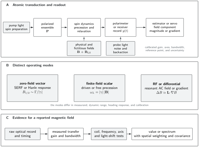
An atomic magnetometer is a calibrated spin-dynamics experiment. A: pump light prepares polarization, the physical and fictitious fields drive spin evolution, and probe light converts that state into an estimator. B: zero-field vector, finite-field scalar, and RF or differential modes have different measurands and operating ranges. C: a reported field requires the raw optical record, measured transfer function, calibration and light-shift tests, spatial weighting, and covariance.

Magnetometer Architectures

Zero-field dispersive magnetometer

The steady-state $P_y(B_x)$ response above is the prototype of a near-zero-field vector channel. The instrument is operated near $B_x=B_y=B_z=0$ using magnetic shields, compensation coils, or feedback. A transverse component tips the pumped polarization and produces optical rotation.

Advantages include a direct odd response around zero and no need to track a high carrier frequency. Limitations include a narrow linear range, cross-axis coupling, sensitivity to coil offsets, and ambiguity if several components are large simultaneously. Three-axis operation generally uses orthogonal modulation fields, multiple optical geometries, or feedback that nulls each component.

Driven finite-field resonance

In an Mx-type magnetometer, circular light prepares polarization and an RF field drives transverse spin resonance. In a Bell–Bloom magnetometer, modulated pump light drives spin precession when the modulation frequency matches the Larmor frequency.

A linear complex response near resonance can be written

$$\chi(\omega) = \frac{ \chi_0 }{ \Gamma_2-i(\omega-\omega_L) }.$$

Its phase is

$$\phi(\omega) = \tan^{-1} \left[ \frac{ \omega-\omega_L }{\Gamma_2} \right]$$

up to the instrument’s sign and phase origin. A servo can adjust the drive frequency until the quadrature error vanishes, yielding

$$\widehat B = \frac{ \widehat\omega_{\mathrm{lock}} }{|\gamma|}.$$

The resonant architecture can operate at much larger fields than a zero-field sensor. It inherits RF coil calibration, Bloch–Siegert shifts, drive-phase delays, and line-center systematics.

Free-precession magnetometer

A pulsed instrument optically pumps the ensemble, turns the pump off, and records a free-induction signal:

$$y(t) = A e^{-t/T_2^*} \cos \left( \omega_Lt+\phi \right) + c + \epsilon(t).$$

The dark interval suppresses pump light shifts and permits frequency estimation from phase accumulation. The estimator must handle finite record length, colored noise, multicomponent Zeeman beats, phase transients, and cycle-to-cycle dead time. A high signal-to-noise sinusoid does not justify a single-frequency model when nonlinear Zeeman components are resolved.

RF atomic magnetometer

An RF magnetometer applies a bias field so an atomic Zeeman transition is resonant with the AC field of interest. The signal estimates an amplitude and phase in a narrow band:

$$\widetilde y(\omega) = H_{yB}(\omega) \widetilde B_{\mathrm{RF}}(\omega) + \widetilde n(\omega).$$

Tuning the bias field changes the center frequency. Narrow bandwidth rejects broadband noise but also distorts pulses or modulated signals outside the calibrated response. RF magnetometers are useful for low-field NMR and nuclear quadrupole resonance, but are not broadband DC vector sensors.

Scalar versus vector operation

Scalar operation derives $|\mathbf B|$ from a precession frequency and can be relatively insensitive to gain drift. Vector operation derives components from amplitudes, phases, or feedback currents and requires calibrated axes.

Scalar does not mean orientation independent. Optical pumping and nonlinear Zeeman structure create heading error. Vector does not mean all three components are independently observable. The response matrix must have full rank:

$$\mathbf y = \mathbf G\mathbf B + \mathbf b + \boldsymbol\epsilon.$$

The condition number of $\mathbf G$ determines how calibration and noise are amplified during inversion.

Differential and array operation

For two sensors,

$$\Delta y = y_2-y_1.$$

Let their gains be

$$G_{1,2} = \overline G \mp \frac{\delta G}{2},$$

and their fields

$$B_{1,2} = \overline B \mp \frac{\Delta B}{2}.$$

Then

$$\Delta y = \overline G\,\Delta B + \delta G\,\overline B + \Delta b.$$

Gain mismatch leaks the common field into the gradient channel. Frequency-dependent mismatch, different sensitive volumes, axis misalignment, and modulation-coil cross-talk also limit common-mode rejection.

For baseline vector $\mathbf L$ and a slowly varying component,

$$\Delta B_i \simeq \sum_j \frac{\partial B_i}{\partial x_j} L_j.$$

The effective baseline joins the response-weighted sensor locations, not necessarily the package centers.

Spin-Exchange Relaxation-Free Operation

Why spin exchange normally broadens

Alkali atoms collide and exchange electron-spin character at rate

$$R_{\mathrm{SE}} = n \left\langle \sigma_{\mathrm{SE}}v \right\rangle,$$

where $n$ is alkali density. Spin exchange largely conserves total angular momentum, but transfers atoms among hyperfine manifolds with different precession frequencies. At ordinary field and low polarization, this random switching dephases a coherent ensemble and broadens magnetic resonance.

Heating a cell increases atom number and optical depth, which could improve statistical sensitivity, but it also raises $R_{\mathrm{SE}}$. This collision limit historically prevented arbitrary improvement by density.

Motional narrowing at low field

In the spin-exchange relaxation-free, or SERF, regime,

$$R_{\mathrm{SE}} \gg \omega_L.$$

Each atom changes hyperfine character many times during one precession period. The ensemble evolves with an averaged precession rather than dephasing after every collision. At low polarization, a schematic spin-exchange relaxation rate is

$$\Gamma_{\mathrm{SE}} \sim C(I,P) \frac{ \omega_L^2 }{ R_{\mathrm{SE}} },$$

where $C(I,P)$ depends on nuclear spin, polarization, and the measured mode. This scaling, not a universal coefficient, is the important result. The spin-exchange contribution vanishes quadratically toward zero field.

Hyperfine correlations also slow the electron-spin response. Detailed SERF models introduce a nuclear slowing-down factor and a polarization-dependent effective gyromagnetic ratio. Using the bare electron gyromagnetic ratio in a SERF calibration is incorrect.

What SERF does not remove

SERF suppresses one relaxation mechanism. It does not eliminate:

• spin-destruction collisions;
• wall and diffusion relaxation;
• pump and probe power broadening;
• magnetic gradients;
• light shifts;
• radiation trapping;
• photon shot noise and spin-projection noise;
• Johnson magnetic noise from conducting shields and heaters; or
• drift and cross-talk in field-nulling coils.

The small-field condition also limits dynamic range. A large ambient field can take the sensor out of the SERF regime or rotate polarization beyond the linear response. High-sensitivity SERF measurements commonly require magnetic shielding or active cancellation. This makes them excellent for some biomagnetic and fundamental measurements but does not make them automatic replacements for geomagnetic scalar instruments.

Density and temperature tradeoffs

Increasing temperature raises alkali density and $R_{\mathrm{SE}}$, helping reach the SERF condition. It can also:

• raise spin-destruction rate;
• increase optical depth and pump nonuniformity;
• increase required heater power and thermal gradients;
• bring conductive materials and their Johnson noise closer to the cell;
• accelerate coating degradation; and
• make close placement near biological or chemical samples harder.

“Higher density is better” is therefore no more reliable than “longer interrogation is better” in a clock.

Sensitivity, Bandwidth, and Range

Noise-equivalent magnetic field

Let the measured output have transfer function $H_{yB}(\omega)$ from the declared field component to output. The amplitude spectral density of equivalent input magnetic noise is

$$S_B^{1/2}(\omega) = \frac{ S_y^{1/2}(\omega) }{ \left| H_{yB}(\omega) \right| }.$$

A quoted value such as $10\ \mathrm{fT\,Hz^{-1/2}}$ is incomplete without frequency, bandwidth, operating point, spatial configuration, and whether environmental field noise has been subtracted. A gradiometric noise floor is not the same quantity as a single-channel absolute noise floor.

First-order response and bandwidth

A simple spin response is low-pass:

$$H_{yB}(\omega) = \frac{ G_0 }{ 1+i\omega/\Gamma_B }.$$

The $-3\ \mathrm{dB}$ bandwidth is

$$f_{3\mathrm{dB}} = \frac{\Gamma_B}{2\pi}.$$

Increasing relaxation or feedback can increase bandwidth, but often reduces open-loop gain or increases noise. Feedback can extend linear range while moving calibration from the atomic slope to coil gain, electronics, delay, and loop stability.

For a transient field, the relevant question is not only the flat-band noise floor. Phase delay and amplitude roll-off must be deconvolved or included in the signal model.

Spin-projection-noise baseline

For $N$ independent polarized spins with coherent interrogation time $T_2$, an order-of-magnitude continuous sensitivity is

$$\eta_B^{(\mathrm{SPN})} \equiv \delta B\sqrt{\tau} \sim \frac{ 1 }{ |\gamma| \sqrt{NT_2} }.$$

Order-one factors depend on spin, polarization, duty cycle, measured quadrature, and estimator. Spin exchange creates correlations that can modify simple independent-spin spectra. Entanglement or squeezing can improve the projection-noise term, but cannot remove a light-shift drift or coil-calibration error.

Photon shot noise and backaction

For optical rotation with slope $d\theta/dB$,

$$\eta_B^{(\mathrm{PSN})} = \frac{ S_\theta^{1/2} }{ \left| d\theta/dB \right| }.$$

More probe photons reduce $S_\theta^{1/2}$ but perturb the atoms more strongly. The optimum balances photon shot noise, spin noise, power broadening, and light shifts under the actual optical-depth model.

Technical noise can enter through:

• laser intensity, frequency, polarization, and pointing;
• photodetector electronics and digitization;
• heater current and modulation;
• coil-current noise;
• mechanical motion through magnetic gradients;
• shield vibration and remanence;
• nearby electronics and mains harmonics; and
• data-acquisition clock jitter.

A noise budget should measure transfer coefficients rather than merely list possible sources.

Dynamic range and linearity

For the zero-field dispersive model, the characteristic linear scale is

$$B_{1/2} = \frac{\Gamma}{|\gamma|}.$$

The exact acceptable range depends on the allowed nonlinearity. If the full response is

$$P_y(B) = \frac{ A B }{ B_{1/2}^2+B^2 },$$

then the ratio to its linear approximation is

$$\frac{ P_y(B) }{ P_y^{(\mathrm{lin})}(B) } = \frac{ 1 }{ 1+(B/B_{1/2})^2 }.$$

Keeping gain error below $1\%$ requires approximately

$$|B| \lesssim 0.10 B_{1/2}.$$

Sensitivity, bandwidth, and linear dynamic range are coupled through $\Gamma$. Quoting only the best noise floor conceals this design tradeoff.

Stability and drift

Allan deviation or overlapping Allan deviation can characterize a stationary field estimate. The result combines sensor drift and real field variation unless a stable source or differential channel separates them. Pump detuning, cell temperature, coil offset, shield magnetization, and laser polarization can create long-term floors.

A flat long-term scalar frequency record does not prove vector-axis stability. A vector sensor can rotate physically while maintaining its component gain.

Calibration and Systematic Effects

Measurement equation

A component channel can be represented as

$$y(t) = y_0 + h \mathbin{*} \left[ B_{\mathrm m} + B_{\mathrm{coil}} + B_{\mathrm{LS}} + B_{\mathrm{contact}} + B_{\mathrm{other}} \right](t) + n(t),$$

where $h$ is the impulse response and $*$ denotes convolution. The target measurand $B_{\mathrm m}$ is accompanied by:

• applied calibration and feedback fields;
• pump and probe light shifts;
• contact or magnetization fields from nearby polarized matter; and
• other physical or instrumental nuisance fields.

The inverse estimator must use the same axis, sign, delay, and bandwidth conventions as the forward model.

Coil calibration

For a calibration coil,

$$B_{\mathrm{coil}} = C_I I,$$

where $C_I$ is the coil factor and $I$ the current. The standard uncertainty is

$$\begin{aligned} u^2(B_{\mathrm{coil}}) ={}& I^2u^2(C_I) + C_I^2u^2(I) \\ &+ 2C_II \operatorname{cov}(C_I,I). \end{aligned}$$

$C_I$ depends on winding geometry, sensor location and orientation, nearby magnetic material, shield response, frequency, and current return path. Calculating an ideal Helmholtz factor is not enough when the coil is inside a high-permeability shield.

Useful calibration routes include:

• dimensional and current calibration of a characterized coil;
• comparison with an independently calibrated magnetometer;
• frequency calibration using a validated gyromagnetic model;
• mechanical rotation in a known field;
• injected AC fields across the measurement bandwidth; and
• reversal of current and sensor orientation.

The routes can share common inputs and should not be assumed independent.

Axis and response-matrix calibration

For a vector instrument,

$$\mathbf y = \mathbf G \left( \mathbf B+\mathbf B_0 \right) + \mathbf b.$$

The matrix $\mathbf G$ contains gains, nonorthogonality, and cross-axis response. Calibrate it by applying several noncoplanar fields whose amplitudes and directions are known. A least-squares fit should include coil-field covariance and residual background.

Sensor axes can vary with pump and probe alignment, modulation phase, and operating point. Package fiducials are not necessarily magnetic axes.

Heading error

A scalar heading test rotates the sensor relative to a field of constant magnitude. The heading error is

$$\Delta B_{\mathrm{head}} \left( \widehat{\mathbf B} \right) = \widehat B_{\mathrm{reported}} \left( \widehat{\mathbf B} \right) - B_{\mathrm{true}}.$$

Sources include:

• nonlinear Zeeman splitting and orientation-dependent line weights;
• unresolved contributions from both hyperfine manifolds;
• light shifts whose direction follows the optical axis;
• RF polarization and Bloch–Siegert shifts;
• cell and coil anisotropy;
• dead zones where pumping or detection vanishes; and
• fitting one line to a changing multicomponent spectrum.

Testing only two opposite headings can miss even angular harmonics. Characterization should cover the solid angle relevant to operation and repeat at several fields, temperatures, and pump powers.

Light-shift and power extrapolation

Reverse pump helicity, change detuning, vary optical power, and introduce dark evolution to separate light shifts. A linear extrapolation to zero power is credible only if the measured range is linear and the zero-power intercept refers to the same atomic state and estimator.

Pump and probe changes can alter polarization, line weights, temperature, and signal-to-noise ratio at the same time. A global model with these nuisance changes is stronger than a one-variable correction.

Gradients, motion, and diffusion

Atoms moving through a nonuniform field accumulate different phases. In a ballistic or diffusive cell, this produces relaxation, line distortion, and a response-weighted location. Motion of the whole sensor through a static gradient produces a time-dependent field:

$$\delta B(t) \simeq \boldsymbol\nabla B \mathbin{\cdot} \delta\mathbf r(t).$$

This is central in wearable biomagnetism and mobile geomagnetic sensing. An accelerometer or optical tracker can aid artifact modelling, but requires calibrated time alignment and a measured field map.

Magnetic shields and Johnson noise

High-permeability shields reduce ambient field and gradient but introduce:

• remanent field and hysteresis;
• temperature-dependent permeability;
• magnetic viscosity and slow relaxation;
• vibration-to-field coupling;
• Johnson-current magnetic noise from conductive layers; and
• altered calibration-coil geometry.

Demagnetization procedures and waiting time should be documented. Environmental noise measured outside the sensor is not automatically the noise inside the shield, and vice versa.

Array cross-talk

Each OPM in an array can produce modulation, compensation, heater, and feedback fields seen by neighboring sensors. Optical beams can also leak between channels. A linear array model is

$$\mathbf y = \mathbf G \left( \mathbf B_{\mathrm{sig}} + \mathbf C\mathbf u \right) + \mathbf b + \boldsymbol\epsilon,$$

where $\mathbf u$ contains all channel control currents and $\mathbf C$ is the coil cross-talk matrix. Measure $\mathbf C$ with each channel driven separately and test whether it depends on frequency, orientation, or shield state.

Uncertainty and covariance

Let the reported field be

$$\widehat B = f \left( \widehat y, \widehat{\mathbf c}, \widehat{\mathbf x} \right),$$

where $\mathbf c$ contains calibration parameters and $\mathbf x$ environmental inputs. First-order propagation gives

$$u^2(B) = \mathbf J \boldsymbol\Sigma \mathbf J^{\mathsf T},$$

where

$$\mathbf J = \frac{\partial f} {\partial (y,\mathbf c,\mathbf x)}.$$

Covariance is common in arrays because channels share lasers, shields, clocks, field coils, and environmental models. Treating every channel and systematic as independent can substantially understate uncertainty in a source reconstruction or gradient.

Validation and Reporting

Transfer-function validation

Inject sinusoidal fields over amplitude and frequency. For each axis, measure:

$$\left| H_{yB}(\omega) \right|, \qquad \arg H_{yB}(\omega).$$

Repeat at representative field offsets, temperatures, pump powers, and orientations. A single small-signal calibration at $10\ \mathrm{Hz}$ does not validate a transient measurement at $100\ \mathrm{Hz}$ or a field near the edge of range.

Null tests and reversals

Useful tests include:

• reverse calibration-coil current;
• reverse pump helicity;
• reverse or block the probe;
• interchange sensor channels;
• rotate the sensor by $180^\circ$ and through a full heading scan;
• vary pump and probe detuning and power;
• vary alkali density and cell temperature;
• inject common and differential fields;
• repeat with dark free-precession readout; and
• compare with an independent sensor technology.

Each test isolates only effects with the corresponding parity. Helicity reversal can reverse both true spin response and vector light shift, so it does not automatically distinguish them.

Minimum report

A comparison-ready magnetometer result should identify:

1. the measurand: component, magnitude, gradient, or spectrum;
2. sensor isotope, manifold, gyromagnetic convention, and field regime;
3. physical reference point, sensitive volume, axis, and spatial weighting;
4. pump, probe, modulation, and feedback configuration;
5. bandwidth, phase delay, sampling, filtering, and dead time;
6. noise-equivalent field as a function of frequency;
7. linear range, saturation, recovery, and heading dependence;
8. coil, frequency, and axis calibration routes;
9. light-shift, gradient, shield, temperature, and cross-talk corrections;
10. statistical and systematic uncertainty with covariance; and
11. raw records, control currents, environmental channels, exclusions, and validation tests.

The phrase “sensitivity of $x\ \mathrm{fT\,Hz^{-1/2}}$” is not a complete instrument specification.

Applications

Biomagnetism

Magnetocardiography and magnetoencephalography detect fields generated by bioelectric currents. OPMs can operate without a cryogenic dewar and can be placed close to the body. The benefit is application specific: sensor noise, standoff distance, channel count, bandwidth, source geometry, shielding, and motion artifacts all matter.

Wearable MEG illustrates the full measurement problem. Movement changes the sensor’s location and orientation in a residual field and gradient, often producing artifacts much larger than the neural signal. Active field nulling, accurate sensor tracking, array calibration, reference channels, and source-reconstruction covariance are part of the instrument, not optional post-processing.

A magnetic map is not a direct image of neural current. The inverse source problem is nonunique and requires anatomical, geometrical, and statistical assumptions.

Low-field NMR and MRI

Atomic magnetometers can detect nuclear free-induction fields where inductive pickup coils become inefficient. Prepolarization, encoding, and detection can occur in separate regions. Near zero field, spectra are often governed by spin–spin $J$ couplings rather than high-field chemical shifts.

The atomic sensor can perturb the sample through bias and modulation coils, and polarized noble gases can produce enhanced contact fields in alkali vapor. The sample–sensor distance, thermal isolation, field homogeneity, and transfer geometry belong in the sensitivity claim.

Geophysics and navigation

Earth-field scalar magnetometers are used for surveys, observatories, space measurements, and anomaly detection. Relevant requirements include:

• operation at fields of order tens of microtesla;
• low heading error over vehicle attitude;
• large dynamic range and fast recovery;
• stable frequency estimation under vibration;
• platform magnetic cleanliness;
• calibrated location and timing; and
• separation of temporal geomagnetic variation from spatial anomalies.

A shielded SERF noise record near zero field does not establish these properties. Finite-field scalar and free-precession architectures are often better matched to geomagnetic operation.

RF sensing and communication

An RF atomic magnetometer can be tuned to a carrier or resonance and detect amplitude, phase, and modulation. Narrowband gain can make weak signals visible, including those used in low-frequency communication or nuclear quadrupole resonance.

Performance should be reported as a transfer function, noise spectrum, linearity, and intermodulation response. A strong nearby carrier can shift or saturate the atomic resonance even when the desired sideband is weak.

Materials and magnetic imaging

Atomic-vapor cells, cold-atom clouds, and solid-state spins can map fields from magnetized rocks, currents, magnetic particles, superconductors, and mesoscopic samples. Spatial resolution is set by sensor–sample distance, sensitive-volume size, field propagation, and inversion, not detector pixel size alone.

NV-center magnetometry can place spins nanometres to micrometres from a sample and operate over broad conditions. Vapor-cell magnetometers can provide excellent field sensitivity over larger volumes. These are different points in a sensitivity–bandwidth–distance–resolution space, not a single ranking.

Fundamental and comagnetometer measurements

Two spin species can occupy nearly the same volume. A weighted difference of their precession frequencies can reject ordinary magnetic-field noise:

$$\Omega_{\mathrm{co}} = \omega_1 - \frac{\gamma_1}{\gamma_2} \omega_2.$$

The cancellation is exact only for identical spatial weighting and well-known gyromagnetic ratios. Species-dependent gradients, contact fields, wall shifts, light shifts, and backaction remain. Such comagnetometers can test rotations, symmetry-violating interactions, or exotic spin couplings, but the interpretation belongs to a declared physical model.

Choosing a platform

Requirement	Often suitable	Principal cautions
shielded low-frequency field component	SERF OPM	narrow range, residual fields, light shifts
Earth’s-field magnitude	scalar driven or free-precession OPM	heading error, nonlinear Zeeman structure
narrowband RF field	tuned RF atomic magnetometer	bandwidth, drive shifts, saturation
near-body multichannel biomagnetism	compact OPM array	motion, cross-talk, thermal and geometric constraints
nanoscale proximity	defect-spin magnetometer	surface noise, readout contrast, calibration
common-mode rejection	atomic gradiometer or array	gain and phase mismatch, baseline definition
field-independent frequency comparison	comagnetometer	species-dependent weighting and contact shifts

A Trustworthy Workflow

Before data collection

1. Define the measurand, axis or magnitude, frequency band, spatial weighting, and reference point.
2. Select the Zeeman model and document isotope, hyperfine state, and gyromagnetic sign.
3. Write the full optical, spin, coil, and estimator forward model.
4. Establish transfer-function, range, and heading requirements from the application.
5. Plan independent coil, frequency, and axis calibrations.
6. Predefine filtering, line fitting, saturation rejection, and uncertainty propagation.

During data collection

Record:

• raw photodiode channels and total optical power;
• pump and probe frequency, power, polarization, and timing;
• cell temperature and heater state;
• all coil currents, feedback values, and modulation phases;
• sensor position and orientation when relevant;
• shield state and demagnetization history;
• calibration injections and reference-sensor channels;
• saturation, relock, and cycle-quality flags; and
• a common timestamp for every channel.

After data collection

1. apply the measured complex transfer function;
2. reconstruct axes or gradients with the calibrated response matrix;
3. propagate coil, gyromagnetic, position, orientation, and cross-talk covariance;
4. inspect residuals against optical, thermal, motion, and control channels;
5. test reversal parities and heading harmonics;
6. distinguish environmental magnetic noise from intrinsic sensor noise;
7. report the valid frequency and amplitude range; and
8. compare with an independent configuration or sensor where the claim warrants it.

Common Mistakes

Treating the Larmor formula as the full instrument

$\omega_L=|\gamma|B$ is the leading transduction law. The measured frequency can be shifted or line-pulled, and the detector averages a finite, possibly nonuniform volume.

Calling a scalar magnetometer orientation independent

The energy magnitude may be rotationally invariant at leading order, but optical pumping, nonlinear Zeeman structure, RF polarization, dead zones, and fitting weights depend on heading.

Equating a noise floor with uncertainty

A spectral noise floor describes fluctuations under stated conditions. Calibration, offset, light shifts, spatial weighting, heading error, and model bias determine measurement uncertainty.

Quoting the gradiometer floor as single-sensor sensitivity

Differencing can reject environmental common mode. It can also hide correlated sensor noise. Report both channel spectra, differential spectrum, baseline, matching, and common-mode transfer.

Assuming SERF means relaxation free

SERF suppresses spin-exchange relaxation in a low-field, fast-exchange regime. Other relaxation and noise remain, and operation outside the near-zero-field range restores spin-exchange broadening.

Increasing laser power without a backaction budget

More power can improve optical shot noise while broadening the resonance, creating light shifts, changing polarization, and adding technical noise.

Using package axes as magnetic axes

The sensitive axes follow optical geometry, modulation, coils, and the operating point. They must be calibrated against fields of known direction.

Ignoring motion through gradients

A stationary field map becomes a time-dependent artifact when the sensor moves. This can dominate wearable or mobile measurements even if the intrinsic sensor noise is very low.

Further Links

• Zeeman Effect in Atoms for Landé factors, Breit–Rabi energies, and field-regime transitions.
• Larmor Precession for the canonical spin-dynamics derivation.
• Magnetic Resonance Overview for driven and pulsed spectroscopy, relaxation, NMR, and EPR.
• Optical Bloch Equations for driven-dissipative optical response and multilevel extensions.
• Atomic Selection Rules for polarization, branching, and magnetic-sublevel transitions.
• Quantum Sensing for information bounds, backaction, and decoherence.
• NV Centers and Solid-State Defects for defect-spin magnetometry and relaxometry.
• NV-Center Sensing for end-to-end NV photon likelihoods, pulse protocols, spatial transfer, vector reconstruction, and nanoscale NMR evidence.
• Spin Coherent States for collective-spin geometry and projection noise.
• Precision Measurement and Metrology for covariance, traceability, and systematic validation.
• Tests of Fundamental Symmetries for electric-odd magnetic backgrounds, comagnetometer mismatch, EDM reversal channels, and particle-physics interpretation.
• Fundamental Symmetry Frontiers for the dated status of comagnetometer, spin-amplifier, axion-mediated, and other spin-dependent interaction searches.

References

1. D. Budker and M. Romalis, “Optical magnetometry,” Nature Physics 3, 227–234 (2007).
2. W. Happer, “Optical pumping,” Reviews of Modern Physics 44, 169–249 (1972).
3. W. E. Bell and A. L. Bloom, “Optical detection of magnetic resonance in alkali metal vapor,” Physical Review 107, 1559–1565 (1957).
4. W. E. Bell and A. L. Bloom, “Optically driven spin precession,” Physical Review Letters 6, 280–281 (1961).
5. D. Budker, W. Gawlik, D. F. Kimball, S. M. Rochester, V. V. Yashchuk, and A. Weis, “Resonant nonlinear magneto-optical effects in atoms,” Reviews of Modern Physics 74, 1153–1201 (2002).
6. W. Happer and H. Tang, “Spin-exchange shift and narrowing of magnetic resonance lines in optically pumped alkali vapors,” Physical Review Letters 31, 273–276 (1973).
7. W. Happer and A. C. Tam, “Effect of rapid spin exchange on the magnetic-resonance spectrum of alkali vapors,” Physical Review A 16, 1877–1891 (1977).
8. I. M. Savukov and M. V. Romalis, “Effects of spin-exchange collisions in a high-density alkali-metal vapor in low magnetic fields,” Physical Review A 71, 023405 (2005).
9. J. C. Allred, R. N. Lyman, T. W. Kornack, and M. V. Romalis, “High-sensitivity atomic magnetometer unaffected by spin-exchange relaxation,” Physical Review Letters 89, 130801 (2002).
10. I. K. Kominis, T. W. Kornack, J. C. Allred, and M. V. Romalis, “A subfemtotesla multichannel atomic magnetometer,” Nature 422, 596–599 (2003).
11. H. B. Dang, A. C. Maloof, and M. V. Romalis, “Ultrahigh sensitivity magnetic field and magnetization measurements with an atomic magnetometer,” Applied Physics Letters 97, 151110 (2010).
12. D. Sheng, S. Li, N. Dural, and M. V. Romalis, “Subfemtotesla scalar atomic magnetometry using multipass cells,” Physical Review Letters 110, 160802 (2013).
13. V. Shah, S. Knappe, P. D. D. Schwindt, and J. Kitching, “Subpicotesla atomic magnetometry with a microfabricated vapour cell,” Nature Photonics 1, 649–652 (2007).
14. S. J. Seltzer and M. V. Romalis, “Unshielded three-axis vector operation of a spin-exchange-relaxation-free atomic magnetometer,” Applied Physics Letters 85, 4804–4806 (2004).
15. W. Lee, V. G. Lucivero, M. V. Romalis, M. E. Limes, E. L. Foley, and T. W. Kornack, “Heading errors in all-optical alkali-vapor magnetometers in geomagnetic fields,” Physical Review A 103, 063103 (2021).
16. I. M. Savukov and M. V. Romalis, “NMR detection with an atomic magnetometer,” Physical Review Letters 94, 123001 (2005).
17. I. M. Savukov, S. J. Seltzer, M. V. Romalis, and K. L. Sauer, “Tunable atomic magnetometer for detection of radio-frequency magnetic fields,” Physical Review Letters 95, 063004 (2005).
18. S. Xu et al., “Magnetic resonance imaging with an optical atomic magnetometer,” Proceedings of the National Academy of Sciences 103, 12668–12671 (2006).
19. E. Boto et al., “Moving magnetoencephalography towards real-world applications with a wearable system,” Nature 555, 657–661 (2018).
20. T. M. Tierney et al., “Optically pumped magnetometers: From quantum origins to multi-channel magnetoencephalography,” NeuroImage 199, 598–608 (2019).
21. J. F. Barry et al., “Sensitivity optimization for NV-diamond magnetometry,” Reviews of Modern Physics 92, 015004 (2020).
22. C. L. Degen, F. Reinhard, and P. Cappellaro, “Quantum sensing,” Reviews of Modern Physics 89, 035002 (2017).
23. A. Fabricant, I. Novikova, and G. Bison, “How to build a magnetometer with thermal atomic vapor: a tutorial,” New Journal of Physics 25, 025001 (2023).
24. JCGM, Evaluation of measurement data: Guide to the expression of uncertainty in measurement, JCGM 100:2008, corrected version 2010.
25. JCGM, International vocabulary of metrology: Basic and general concepts and associated terms, JCGM 200:2012, third edition.

Exercises

1. Zeeman scale and frequency uncertainty

Use

$$\frac{|\gamma_F|}{2\pi} = 6.998\ \mathrm{Hz\,nT^{-1}}$$

for the $^{87}\mathrm{Rb}$ $F=2$ manifold.

1. Find the Larmor frequency at $B=50.000\ \mu\mathrm T$.
2. A fit gives $f_L=349\,902.0\ \mathrm{Hz}$ with standard uncertainty $0.8\ \mathrm{Hz}$. Ignoring uncertainty in $\gamma_F$, find $\widehat B$ and its standard uncertainty.
3. If an unmodelled heading shift changes the fitted frequency by $3.5\ \mathrm{Hz}$, express the magnetic bias in nT.

Solution

Convert

$$50.000\ \mu\mathrm T = 50\,000\ \mathrm{nT}.$$

The frequency is

$$\begin{aligned} f_L &= \left( 6.998\ \mathrm{Hz\,nT^{-1}} \right) \left( 50\,000\ \mathrm{nT} \right) \\ &= 349\,900\ \mathrm{Hz}. \end{aligned}$$

The fitted field is

$$\widehat B = \frac{349\,902.0}{6.998}\ \mathrm{nT} \simeq 50\,000.29\ \mathrm{nT} = 50.00029\ \mu\mathrm T.$$

The frequency-fit contribution is

$$u(B) = \frac{0.8}{6.998}\ \mathrm{nT} \simeq 0.114\ \mathrm{nT}.$$

The heading bias is

$$\Delta B_{\mathrm{head}} = \frac{3.5}{6.998}\ \mathrm{nT} \simeq 0.50\ \mathrm{nT}.$$

It is more than four times the statistical standard uncertainty, showing why a precise frequency fit is not the whole uncertainty budget.

2. Zero-field Bloch response

Starting from

$$\frac{d\mathbf P}{dt} = \gamma\mathbf P\times B_x\widehat{\mathbf x} + Rs\widehat{\mathbf z} - \Gamma\mathbf P,$$

derive the steady-state $P_y$ and $P_z$. Find the field half-width and the zero-field slope. For

$$\frac{|\gamma|}{2\pi} = 7.0\ \mathrm{Hz\,nT^{-1}}, \qquad \Gamma=2\pi(100)\ \mathrm{s^{-1}},$$

find $B_{1/2}$.

Solution

For $\mathbf B=B_x\widehat{\mathbf x}$,

$$\mathbf P\times\mathbf B = \begin{pmatrix} 0\\ P_zB_x\\ -P_yB_x \end{pmatrix}.$$

The steady $y$ and $z$ equations are

$$0 = \gamma B_xP_z-\Gamma P_y,$$

and

$$0 = -\gamma B_xP_y+Rs-\Gamma P_z.$$

The first gives

$$P_y = \frac{\gamma B_x}{\Gamma}P_z.$$

Substitution gives

$$P_z = \frac{ Rs\Gamma }{ \Gamma^2+\gamma^2B_x^2 },$$

and

$$P_y = \frac{ Rs\gamma B_x }{ \Gamma^2+\gamma^2B_x^2 }.$$

The half-width is

$$B_{1/2} = \frac{\Gamma}{|\gamma|},$$

and the zero-field slope is

$$\left. \frac{dP_y}{dB_x} \right|_{0} = \frac{Rs\gamma}{\Gamma^2}.$$

Numerically, the factors of $2\pi$ cancel:

$$B_{1/2} = \frac{ 100\ \mathrm{Hz} }{ 7.0\ \mathrm{Hz\,nT^{-1}} } \simeq 14.3\ \mathrm{nT}.$$

The useful range for less than $1\%$ gain error would be only about $1.4\ \mathrm{nT}$ in the simple Lorentzian model.

3. Projection-noise baseline

An ensemble contains $N=1.0\times10^{11}$ effectively measured atoms with $T_2=10\ \mathrm{ms}$ and

$$|\gamma| = 2\pi \left( 7.0\times10^9 \right) \mathrm{rad\,s^{-1}\,T^{-1}}.$$

1. Estimate $\eta_B^{(\mathrm{SPN})}\sim1/(|\gamma|\sqrt{NT_2})$.
2. If contrast and duty cycle together worsen the field noise by a factor $3$, find the adjusted baseline.
3. An observed noise floor is $12\ \mathrm{fT\,Hz^{-1/2}}$. By what factor does it exceed the adjusted baseline?

Solution

First,

$$\sqrt{NT_2} = \sqrt{ (1.0\times10^{11})(1.0\times10^{-2}) } = \sqrt{10^9} \simeq 3.162\times10^4\ \mathrm{s^{1/2}}.$$

The gyromagnetic ratio is

$$|\gamma| \simeq 4.398\times10^{10}\ \mathrm{rad\,s^{-1}\,T^{-1}}.$$

Therefore

$$\eta_B^{(\mathrm{SPN})} \sim \frac{1}{ (4.398\times10^{10})(3.162\times10^4) } \simeq 7.2\times10^{-16}\ \mathrm{T\,Hz^{-1/2}}.$$

Thus

$$\eta_B^{(\mathrm{SPN})} \simeq 0.72\ \mathrm{fT\,Hz^{-1/2}}.$$

Including the factor of three gives

$$\eta_B^{(\mathrm{adj})} \simeq 2.16\ \mathrm{fT\,Hz^{-1/2}}.$$

The measured floor is higher by

$$\frac{12}{2.16} \simeq 5.6.$$

The estimate is an order-of-magnitude baseline. A rigorous comparison requires the actual polarization, spin quantum number, correlations, readout efficiency, and estimator.

4. Coil calibration with covariance

A coil has

$$C_I = (50.00\pm0.10)\ \mathrm{nT\,mA^{-1}},$$

and is driven at

$$I = (2.000\pm0.004)\ \mathrm{mA}.$$

The correlation coefficient between fitted $C_I$ and current calibration is $\rho=-0.40$.

1. Find the applied field.
2. Find its standard uncertainty including covariance.
3. Compare with the uncertainty obtained by assuming independence.

Solution

The field is

$$B = C_II = (50.00)(2.000)\ \mathrm{nT} = 100.00\ \mathrm{nT}.$$

The covariance is

$$\operatorname{cov}(C_I,I) = \rho\,u(C_I)u(I) = (-0.40)(0.10)(0.004) = -1.6\times10^{-4}\ \mathrm{nT}.$$

Using units consistent with $C_I I$,

$$\begin{aligned} u^2(B) ={}& I^2u^2(C_I) + C_I^2u^2(I) \\ &+ 2C_II\operatorname{cov}(C_I,I) \\ =& (2.000)^2(0.10)^2 + (50.00)^2(0.004)^2 \\ &+ 2(50.00)(2.000) (-1.6\times10^{-4}) \\ =& 0.040+0.040-0.032 \\ =& 0.048\ \mathrm{nT^2}. \end{aligned}$$

Therefore

$$u(B) \simeq 0.219\ \mathrm{nT}.$$

Ignoring covariance gives

$$u_{\rho=0}(B) = \sqrt{0.080}\ \mathrm{nT} \simeq 0.283\ \mathrm{nT}.$$

The negative covariance reduces the propagated uncertainty. It must be supported by the joint calibration fit rather than chosen to improve the budget.

5. SERF criterion and narrowing

An alkali vapor has spin-exchange rate

$$R_{\mathrm{SE}} = 2.0\times10^5\ \mathrm{s^{-1}}$$

and effective

$$\frac{|\gamma|}{2\pi} = 7.0\ \mathrm{Hz\,nT^{-1}}.$$

Use the schematic estimate

$$\Gamma_{\mathrm{SE}} \simeq \frac{\omega_L^2}{R_{\mathrm{SE}}}$$

with coefficient one.

1. Evaluate $\omega_L/R_{\mathrm{SE}}$ and $\Gamma_{\mathrm{SE}}$ at $B=1.0\ \mathrm{nT}$.
2. Repeat at $B=1.0\ \mu\mathrm T$.
3. Explain the domain of this estimate.

Solution

At $1.0\ \mathrm{nT}$,

$$\omega_L = 2\pi(7.0) \simeq 44.0\ \mathrm{s^{-1}}.$$

Thus

$$\frac{\omega_L}{R_{\mathrm{SE}}} \simeq 2.2\times10^{-4} \ll 1,$$

and

$$\Gamma_{\mathrm{SE}} \simeq \frac{(44.0)^2}{2.0\times10^5} \simeq 9.7\times10^{-3}\ \mathrm{s^{-1}}.$$

At $1.0\ \mu\mathrm T=1000\ \mathrm{nT}$,

$$\omega_L \simeq 4.40\times10^4\ \mathrm{s^{-1}},$$

so

$$\frac{\omega_L}{R_{\mathrm{SE}}} \simeq 0.22.$$

The fast-exchange separation is much weaker, and the schematic expression would give

$$\Gamma_{\mathrm{SE}} \simeq \frac{(4.40\times10^4)^2}{2.0\times10^5} \simeq 9.7\times10^3\ \mathrm{s^{-1}}.$$

The quadratic estimate is an asymptotic low-field scaling with a species-, polarization-, and mode-dependent coefficient. It should not be used quantitatively when $\omega_L/R_{\mathrm{SE}}$ is no longer small; the coupled hyperfine spin-exchange dynamics must then be solved.

6. Gradiometer gain mismatch

Two OPM channels have mean gain $\overline G=1.00\ \mathrm{V\,nT^{-1}}$ and relative mismatch

$$\frac{\delta G}{\overline G} = 3.0\times10^{-4}.$$

They measure a common background $\overline B=40\,000\ \mathrm{nT}$ and a true differential signal $\Delta B=0.50\ \mathrm{nT}$.

1. Find the desired differential output.
2. Find the common-field leakage.
3. What relative matching is required to keep leakage below $0.05\ \mathrm{nT}$ equivalent field?

Solution

The desired output is

$$\Delta y_{\mathrm{sig}} = \overline G\Delta B = 0.50\ \mathrm V.$$

The gain difference is

$$\delta G = (3.0\times10^{-4}) (1.00\ \mathrm{V\,nT^{-1}}) = 3.0\times10^{-4}\ \mathrm{V\,nT^{-1}}.$$

The leaked output is

$$\Delta y_{\mathrm{leak}} = \delta G\overline B = (3.0\times10^{-4})(40\,000) = 12\ \mathrm V.$$

This is equivalent to $12\ \mathrm{nT}$ at the mean gain, far larger than the signal. To keep the equivalent leakage below $0.05\ \mathrm{nT}$,

$$\frac{\delta G}{\overline G} < \frac{0.05}{40\,000} = 1.25\times10^{-6}.$$

In practice a geomagnetic gradiometer often estimates and subtracts channel gains continuously or operates scalar frequency channels. Axis and frequency-response mismatch remain.

7. Heading-parity model

A scalar magnetometer has heading error

$$\Delta B(\theta) = a_0 + a_1\cos\theta + b_1\sin\theta + a_2\cos2\theta.$$

Measurements at $\theta=0,\pi/2,\pi,3\pi/2$ give, in nT,

$$\begin{array}{c|rrrr} \theta &0&\pi/2&\pi&3\pi/2\\ \hline \Delta B &1.8&-0.4&-0.2&0.8 \end{array}.$$

Find $a_0$, $a_1$, $b_1$, and $a_2$. Why would measurements only at $0$ and $\pi$ be insufficient?

Solution

The four equations are

$$\begin{aligned} 1.8 &= a_0+a_1+a_2, \\ -0.4 &= a_0+b_1-a_2, \\ -0.2 &= a_0-a_1+a_2, \\ 0.8 &= a_0-b_1-a_2. \end{aligned}$$

Adding all four gives

$$4a_0 = 2.0,$$

so

$$a_0 = 0.50\ \mathrm{nT}.$$

The opposite-heading differences give

$$a_1 = \frac{1.8-(-0.2)}{2} = 1.00\ \mathrm{nT},$$

and

$$b_1 = \frac{-0.4-0.8}{2} = -0.60\ \mathrm{nT}.$$

Using the first equation,

$$a_2 = 1.8-0.50-1.00 = 0.30\ \mathrm{nT}.$$

Measurements only at $0$ and $\pi$ determine $a_1$ and the combination $a_0+a_2$, but cannot separate the constant and even second harmonic. They also provide no information about $b_1$. Opposite-heading reversal is not a complete heading characterization.

8. Design an OPM-MEG validation

A laboratory plans a 32-channel wearable OPM-MEG system. Each sensor has a manufacturer noise specification of $10\ \mathrm{fT\,Hz^{-1/2}}$ from $3$ to $100\ \mathrm{Hz}$ and a nominal linear range of $\pm1.5\ \mathrm{nT}$. Design a validation and reporting program before neural source-localization claims are made. Address the measurand, field nulling, motion, array calibration, cross-talk, timing, noise, source validation, covariance, and participant safety.

Solution

A defensible program could include:

1. Measurand and geometry. Define each measured component in a head-fixed or room-fixed frame, record sensor sensitive axes and response-weighted locations, and document how those quantities enter the forward source model.
2. Magnetic environment. Map static field and gradients over the full head-motion volume. Validate active nulling, its bandwidth, coil calibration, residual field, and recovery after saturation. The $\pm1.5\ \mathrm{nT}$ range must be compared with motion through this map, not with the field at one central point.
3. Channel transfer functions. Inject calibrated fields along several axes and measure complex gain, bandwidth, nonlinearity, saturation, and recovery for every sensor in its installed location.
4. Cross-talk. Drive every modulation and compensation coil separately while recording all channels. Fit a frequency-dependent cross-talk matrix and test whether simultaneous operation changes gain.
5. Motion tracking. Calibrate the optical tracking system, sensor-to- marker transformations, latency, and dropped samples. Move a rigid sensor phantom through the measured residual field to validate predicted motion artifacts.
6. Timing. Place sensor, coil-drive, motion, stimulus, and physiology records on a common clock. Inject simultaneous optical and magnetic events to measure channel delays and jitter.
7. Noise. Report installed single-channel and cross-spectral noise, empty-room recordings, reference-channel coherence, mains harmonics, vibration coupling, and drift. Do not substitute the manufacturer’s isolated-sensor specification.
8. Known sources. Use calibrated current dipoles or a head phantom at several locations, orientations, depths, and movement trajectories. Blind the analysis to some source parameters and test localization, amplitude, and uncertainty coverage.
9. Biological repeatability. Reproduce well-established evoked responses with preregistered timing and processing, while separating evidence for sensor performance from neuroscience interpretation.
10. Covariance and inversion. Carry channel gain, axis, location, cross-talk, field-map, and noise covariance into source reconstruction. Report sensitivity to regularization and head-model assumptions.
11. Safety and comfort. Evaluate optical containment, surface temperature, electrical isolation, acoustic and mechanical risks, emergency removal, participant movement, and applicable institutional and medical-device procedures.
12. Audit trail. Retain raw channels, control currents, tracking, calibration data, exclusions, software versions, and shield state for every session.

Only after installed-system validation should the nominal sensor floor be used in a neural-source uncertainty claim.