Tests of Fundamental Symmetries

A fundamental-symmetry test asks whether an observable forbidden by a specified symmetry is consistent with zero, or measures a known symmetry-violating amplitude precisely enough to test its predicted size. Atomic, molecular, and optical systems are valuable because coherent evolution converts very small interactions into phases, while state labels and controlled reversals provide strong diagnostics of ordinary backgrounds.

Two major classes of experiment illustrate the method:

• searches for permanent electric dipole moments (EDMs) test interactions that are odd under parity $P$ and time reversal $T$; and
• atomic parity-violation (APV) measurements isolate weak-interaction amplitudes that are odd under $P$ but, for the dominant weak-charge interaction, even under $T$.

The observable at the detector is not itself a fundamental coupling. A credible result requires an inference chain,

$$\begin{gathered} \text{counts, phases, or frequencies} \longrightarrow \text{reversal channel} \longrightarrow \text{system-level moment or amplitude} \\ \longrightarrow \text{atomic, molecular, or nuclear response} \longrightarrow \text{effective interaction} \longrightarrow \text{particle-physics constraint}. \end{gathered}$$

Each arrow carries calibration, theory, uncertainty, and assumptions. A small confidence interval on a raw frequency does not by itself make the last arrow trustworthy.

Canonical Scope

Parity owns spatial inversion, parity eigenstates, and elementary selection rules. Time Reversal and Antiunitary Time Reversal own the antiunitary operator and its action on states, observables, and dynamics. From Discrete Symmetries to CPT states the assumptions behind the connection among $C$, $P$, $T$, and $CPT$.

Precision Measurement and Metrology owns the general language of measurands, covariance, reversals, calibration, blinding, and uncertainty. Ramsey Interferometry owns the separated-field fringe and phase estimator. Magnetometry owns magnetic-field measurement and calibration. Cold Molecules owns molecular production, cooling, trapping, polarization, and internal state control. Precision Molecular Measurements owns body-to-laboratory orientation, molecular response calibration, electron and nuclear sensor architectures, chiral parity comparisons, and cold-platform precision tradeoffs.

This page owns:

• the symmetry signatures of spin-aligned EDMs and APV amplitudes;
• Ramsey and multi-switch estimators for EDM searches;
• representative current EDM bounds and the assumptions behind them;
• Schiff screening and the distinction among paramagnetic, diamagnetic, neutron, and nuclear probes;
• the weak-charge and nuclear-spin-dependent parts of APV;
• molecules as enhancement and internal-comagnetometer platforms;
• experiment-specific systematic effects and validation tests; and
• the map from AMO observables to effective operators and particle-physics models.

The numerical status statements below are reviewed as of 2026-07-26. They should be rechecked against the current Particle Data Group review and the primary experimental literature before being used in a new analysis.

What a Symmetry Test Measures

Exact transformation, experimental reversal, and null hypothesis

Three operations must not be conflated.

1. A symmetry transformation acts on every relevant state, observable, and external field according to a mathematical rule.
2. An experimental reversal changes a controllable label such as electric-field polarity, molecular orientation, spin projection, laser polarization, or propagation direction.
3. A null hypothesis is a statistical model, including nuisance parameters, under which a chosen symmetry-sensitive coefficient has a specified value, often zero.

Reversing a laboratory electric field is not the antiunitary $T$ operation. It is useful because the desired interaction has a known parity under that switch. The experiment must show that ordinary effects with the same switch parity are absent or bounded.

Polar and axial vectors

The transformation rules needed for the leading EDM argument are

Quantity	Type	Under $P$	Under $T$
Position $\mathbf r$	polar	$-\mathbf r$	$\mathbf r$
Electric field $\mathbf E$	polar	$-\mathbf E$	$\mathbf E$
Momentum $\mathbf p$	polar	$-\mathbf p$	$-\mathbf p$
Angular momentum $\mathbf J$	axial	$\mathbf J$	$-\mathbf J$
Spin $\mathbf S$	axial	$\mathbf S$	$-\mathbf S$
Magnetic field $\mathbf B$	axial	$\mathbf B$	$-\mathbf B$

For a nondegenerate stationary system with angular momentum, rotational covariance permits a permanent vector EDM only along the angular-momentum axis. A convenient effective interaction is

$$H_{\mathrm{EDM}} = -d\, \widehat{\mathbf J} \mathbin{\cdot} \mathbf E,$$

where $\widehat{\mathbf J}$ denotes the oriented angular-momentum axis and $d$ is the corresponding system-level coefficient. Because $\mathbf J\mathbin{\cdot}\mathbf E$ is odd under both $P$ and $T$, a nonzero permanent spin-aligned EDM is a $P$-odd and $T$-odd observable.

Under the usual assumptions of local, Lorentz-invariant quantum field theory, $CPT$ is conserved. Within that framework, $T$ violation implies $CP$ violation. The statement is conditional: an EDM experiment directly tests a $T$-odd interaction in its low-energy Hamiltonian, while the translation to $CP$ uses $CPT$ assumptions.

Known violation and forbidden violation

Parity violation by the weak interaction is established. APV experiments therefore do not generally test the hypothesis that all parity violation is zero. They test whether a measured weak amplitude agrees with the Standard Model after electroweak, nuclear, and atomic-structure corrections.

No permanent EDM of an elementary particle or nondegenerate bound system has been established. EDM searches are therefore null tests whose upper limits constrain combinations of $CP$-odd interactions.

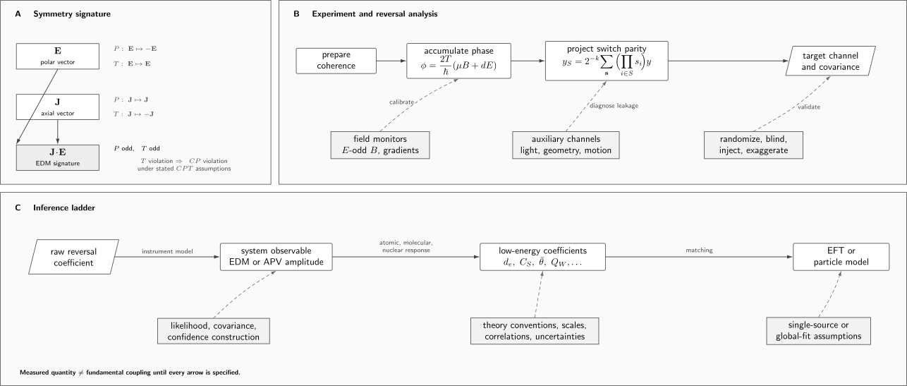
A trustworthy symmetry test separates three layers. The transformation properties identify the target signature; balanced switches isolate a raw channel while auxiliary channels diagnose leakage; response calculations and statistical assumptions then connect the system-level result to effective interactions. No arrow in the inference ladder is automatic.

Electric Dipole Moment Searches

A minimal spin-precession model

Consider two spin projections in collinear electric and magnetic fields. Choose signs so that the effective Hamiltonian is

$$H = -\mu B\,\sigma_z -dE\,\sigma_z.$$

The energy splitting and angular precession frequency are then

$$\hbar\omega(E,B) = 2\mu B +2dE.$$

Only the sign convention changes if the magnetic moment, quantization axis, or state labels are defined differently. The experimentally useful fact is that the EDM term is odd under reversal of the effective electric field, whereas the leading magnetic term is even if $B$ is unchanged.

For nominal electric-field settings $+E$ and $-E$,

$$\begin{aligned} \omega(+E)-\omega(-E) &= \frac{4dE}{\hbar} \\ &\quad+ \frac{2\mu}{\hbar} \left[ B(+E)-B(-E) \right]. \end{aligned}$$

Define the electric-odd magnetic field

$$B_E = \frac{B(+E)-B(-E)}{2}.$$

An estimator that ignores this correlation returns

$$\widehat d = d + \frac{\mu B_E}{E},$$

so the false EDM is

$$d_{\mathrm{false}} = \frac{\mu B_E}{E}.$$

This compact expression explains why magnetic shielding alone is insufficient. Leakage currents, charging transients, coil cross-talk, or motion through a gradient can create a magnetic change correlated with the high-voltage reversal.

Ramsey phase

A Ramsey sequence prepares a coherent superposition, allows it to evolve for time $T$, and converts relative phase into population. In the minimal model,

$$\phi(E,B) = \phi_0 + \frac{2T}{\hbar} \left( \mu B+dE \right).$$

The half-difference under electric reversal is

$$\begin{aligned} \phi_E &\equiv \frac{\phi(+E)-\phi(-E)}{2} \\ &= \frac{2dET}{\hbar} + \frac{2\mu B_E T}{\hbar}. \end{aligned}$$

After independently constraining the magnetic term,

$$\widehat d = \frac{\hbar\phi_E}{2ET}.$$

The estimator is only linear while the phase can be unwrapped and the readout discriminator remains calibrated. Experiments often fit all switch states at once rather than forming pairwise differences, and may use a nearby transition or species as a comagnetometer.

Statistical sensitivity

If the uncertainty of the electric-odd phase after all averaging is $\sigma_{\phi_E}$, then

$$\sigma_d = \frac{\hbar\sigma_{\phi_E}} {2E_{\mathrm{eff}}T}.$$

For projection-noise-limited binary readout with total detected count $N_{\mathrm{det}}$ and contrast $C$, a useful scale is

$$\sigma_d^{\mathrm{SQL}} \sim \frac{\hbar} {2E_{\mathrm{eff}}TC\sqrt{N_{\mathrm{det}}}}.$$

Here $E_{\mathrm{eff}}$ is the field multiplying the targeted EDM coefficient in the effective Hamiltonian. For a free neutron it is the applied field, subject to geometry and field averaging. For an electron EDM in a polar molecule it is a relativistic, molecule-frame effective field obtained from electronic-structure theory. It is not the laboratory polarizing field.

Increasing $E_{\mathrm{eff}}$, $T$, contrast, or detected number improves the statistical scale, but each can change the systematic model. Longer interrogation may amplify geometric phases; stronger polarization fields may increase leakage currents; a denser sample may introduce collisions; and more detected photons may increase light shifts.

Multi-Switch Reversal Analysis

Switch-parity basis

Let $s_i=\pm1$ label $k$ independently controlled switches. Examples include:

• applied electric-field polarity;
• molecular orientation or internal doublet;
• magnetic-field direction;
• spin-precession sense;
• laser propagation direction;
• preparation or readout polarization; and
• detector or analysis channel.

For a measured quantity $y(\mathbf s)$ sampled in every switch configuration, define the coefficient in channel $S$ by

$$y_S = \frac{1}{2^k} \sum_{\mathbf s} \left( \prod_{i\in S}s_i \right) y(\mathbf s).$$

These coefficients are a discrete Walsh expansion:

$$y(\mathbf s) = \sum_S y_S \prod_{i\in S}s_i.$$

The desired EDM signal lies in a known odd channel, but the precise switch product is apparatus dependent. In a molecular experiment the useful “electric” switch may be the sign of the molecule’s internal orientation, not merely the sign of the laboratory voltage.

Why auxiliary channels matter

If every switch is perfectly balanced and independent, distinct parity channels are orthogonal. Real switches change more than their intended sign. Reversing high voltage can change $|E|$, current, beam trajectory, contrast, or trap position. Reversing polarization can change optical power. Missing switch states and time drift also destroy orthogonality.

A linearized model can be written

$$\mathbf y = X\boldsymbol\beta + \boldsymbol\epsilon,$$

where the design matrix $X$ contains switch products, drift terms, and measured nuisance monitors. With covariance $V$,

$$\widehat{\boldsymbol\beta} = \left( X^{\mathsf T}V^{-1}X \right)^{-1} X^{\mathsf T}V^{-1}\mathbf y.$$

The fit should report the design-matrix rank, relevant correlations, and coverage tests. A small target-channel coefficient is not persuasive if a large auxiliary channel can leak through an unmeasured switch imbalance.

Randomization and blinding

Useful protections include:

1. balance switch states over times shorter than important drifts;
2. randomize or pseudorandomize blocks subject to that balance;
3. record actual field magnitudes and transient monitors, not only command bits;
4. define quality cuts without viewing the unblinded target coefficient;
5. inject a concealed offset through a controlled analysis layer;
6. freeze the estimator and uncertainty prescription before unblinding;
7. run null, exaggeration, and signal-injection tests; and
8. preserve both blinded and final analysis trails.

Blinding protects choices from subconscious optimization. It does not validate the physical model or repair an incomplete systematic search.

Which EDM Does a System Probe?

Paramagnetic atoms and molecules

Systems with unpaired electron angular momentum are especially sensitive to electron-sector $P,T$-odd interactions. A schematic molecular spin-precession energy is

$$\Delta E_{P,T} = -\Omega \left( d_e E_{\mathrm{eff}} + C_S W_S + \cdots \right),$$

where:

• $d_e$ is the electron EDM;
• $E_{\mathrm{eff}}$ is the calculated internal effective field;
• $C_S$ is a scalar electron–nucleon coupling in one common normalization;
• $W_S$ is the corresponding molecular response coefficient; and
• $\Omega$ labels the projection of electronic angular momentum on the molecular axis.

Signs and normalization differ across the literature. An experiment measures the combination multiplying its selected levels. Quoting a bound on $d_e$ alone therefore normally imposes the single-source assumption $C_S=0$ and neglects other relevant operators. Combining species with different response vectors can constrain more than one coefficient.

Relativistic mixing in heavy atoms and molecules amplifies the electron-EDM response. The enhancement does not mean that the electron experiences the applied laboratory field as a classical field of the quoted magnitude. $E_{\mathrm{eff}}$ is a matrix-element coefficient and carries electronic-structure uncertainty.

Diamagnetic atoms

Closed-electron-shell atoms such as $^{199}\mathrm{Hg}$ have suppressed direct electron-spin sensitivity. Their EDMs can receive contributions from:

• a nuclear Schiff moment;
• $P,T$-odd nucleon–nucleon interactions;
• nucleon EDMs;
• tensor and scalar-pseudoscalar electron–nucleon interactions; and
• other hadronic or semileptonic operators.

The system EDM is therefore not simply the EDM of its nucleus. Its interpretation requires a chain through atomic, nuclear, and hadronic calculations.

Schiff screening

For a neutral atom made from nonrelativistic point charges interacting electrostatically, a static external field is rearranged so that a pointlike nuclear EDM is screened from the atomic energy at leading order. This is the content of Schiff’s theorem under its stated assumptions.

Real atoms evade complete screening through finite nuclear size, relativistic effects, magnetic interactions, and $P,T$-odd forces. A nuclear Schiff moment $\mathbf S$ is one finite-size source that couples to the electrons. The atomic response is often organized as

$$d_{\mathrm{atom}} = k_S S + \sum_a k_a c_a,$$

where $k_S$ is an atomic-structure coefficient and the remaining $c_a$ represent other low-energy sources. Nuclear structure then relates $S$ to hadronic $CP$-odd couplings. Uncertainties at these different layers must not be collapsed into one unexplained conversion factor.

Neutrons and nuclei

A free-neutron EDM directly concerns a hadron, but its relation to quark EDMs, chromo-EDMs, four-quark operators, and the QCD angle $\overline\theta$ still requires nonperturbative hadronic theory. Nuclear EDM and magnetic-quadrupole-moment searches add collective and deformation-sensitive responses.

The systems are complementary rather than interchangeable:

Probe class	Leading sensitivities in common analyses	Essential theory
Paramagnetic atom or molecule	$d_e$, $C_S$, other electron-sector terms	relativistic atomic or molecular structure
Diamagnetic atom	Schiff moment, hadronic and semileptonic terms	atomic, nuclear, and hadronic structure
Neutron	$\overline\theta$, quark and gluon operators	nonperturbative QCD and hadronic EFT
Polarized nucleus or molecule	nuclear moments and electron–nucleus couplings	molecular, nuclear, and hadronic structure

This classification is a leading-order guide, not a proof that all other sensitivities vanish.

Representative EDM Status

The table lists representative record bounds reviewed on 2026-07-25. All quoted measurements are consistent with zero.

Reported quantity	Representative result or limit	Confidence level	Physical system	Interpretation note
Electron EDM $d_e$	$\lvert d_e\rvert<4.1\times10^{-30}\ e\,\mathrm{cm}$	90%	trapped $^{180}\mathrm{Hf}^{19}\mathrm{F}^{+}$	inferred with other $P,T$-odd sources, especially $C_S$, set to zero
Neutron EDM $d_n$	$\lvert d_n\rvert<1.8\times10^{-26}\ e\,\mathrm{cm}$	90%	stored ultracold neutrons	system-level neutron moment; operator interpretation needs hadronic theory
Atomic EDM $d_{\mathrm{Hg}}$	$\lvert d_{\mathrm{Hg}}\rvert<7.4\times10^{-30}\ e\,\mathrm{cm}$	95%	$^{199}\mathrm{Hg}$ vapor cells	diamagnetic-atom result; commonly mapped through a nuclear Schiff moment

For the HfF$^+$ experiment, the reported single-source estimate was

$$d_e = \left( -1.3 \pm2.0_{\mathrm{stat}} \pm0.6_{\mathrm{syst}} \right) \times10^{-30}\ e\,\mathrm{cm}.$$

The neutron result was

$$d_n = \left( 0.0 \pm1.1_{\mathrm{stat}} \pm0.2_{\mathrm{syst}} \right) \times10^{-26}\ e\,\mathrm{cm},$$

and the mercury result, including its published correction, was

$$d_{\mathrm{Hg}} = \left( -2.20 \pm2.75_{\mathrm{stat}} \pm1.48_{\mathrm{syst}} \right) \times10^{-30}\ e\,\mathrm{cm}.$$

The numerical limits should not be ranked merely by comparing powers of $e\,\mathrm{cm}$. Each system responds to a different combination of low-energy operators with different enhancement, screening, and theory uncertainties.

Time-Reversal Tests in Practice

A laboratory reversal is not time reversal

The antiunitary operation $T$ reverses momenta and angular momenta, complex-conjugates amplitudes, and transforms all $T$-odd external parameters. Flipping one electrode voltage does none of that. The experimental reversal is instead a projector onto a coefficient expected to share the EDM’s sign behavior.

This distinction prevents two common errors:

• an $E$-odd frequency shift is not automatically $T$ violation; and
• failure to reproduce a trajectory backward in time is not evidence for microscopic $T$ violation.

Ordinary dissipative dynamics, state loss, hysteresis, and feedback can make a laboratory sequence look irreversible even when the microscopic Hamiltonian respects $T$.

Motional fields and geometric phases

An object moving with velocity $\mathbf v$ through an electric field sees, to leading nonrelativistic order, a motional magnetic field

$$\mathbf B_{\mathrm{mot}} \simeq -\frac{\mathbf v\times\mathbf E}{c^2}.$$

Its simple ensemble average may vanish, yet correlations with magnetic gradients and wall or trap motion can produce a geometric-phase frequency shift that is odd under electric reversal. A comagnetometer can diagnose field drift but may sample a different spatial distribution and velocity correlation, so it does not automatically cancel this effect.

Validation can require:

• deliberate gradient scans;
• electric-field magnitude scans;
• trajectory or temperature changes;
• species-dependent simulations benchmarked against field maps;
• reversal-rate scans;
• storage-time scans; and
• comparison of cohabiting probes with different kinematics.

Internal comagnetometry

Closely spaced molecular states with opposite orientation can experience nearly the same laboratory magnetic field while reversing the sign of the internal effective electric field. Their frequency difference can strongly reject common magnetic noise. Such an internal comagnetometer is powerful because spatial co-location is excellent.

It is not perfect. The paired states can have different magnetic moments, Stark shifts, transition strengths, geometric phases, or state-dependent trajectories. Those differences must be measured and propagated.

Parity Violation in Atoms

Nuclear-spin-independent weak interaction

At momentum transfers characteristic of an atom, neutral-current electron–nucleus interactions can be represented by a short-range Hamiltonian. One common convention for the nuclear-spin-independent part is

$$H_W^{\mathrm{NSI}} = \sum_i \frac{G_F}{2\sqrt2} Q_W \rho_N(r_i) \gamma_5^{(i)},$$

where $G_F$ is the Fermi constant, $\rho_N$ is a normalized nuclear density, $i$ labels electrons, $\gamma_5^{(i)}$ acts on electron $i$‘s Dirac degrees of freedom, and $Q_W$ is the nuclear weak charge. Overall signs and density normalizations vary by convention.

At tree level, the dominant Standard Model dependence is approximately

$$Q_W \simeq -N + Z \left( 1-4\sin^2\theta_W \right) + \Delta Q_W,$$

where $Z$ and $N$ are proton and neutron numbers and $\Delta Q_W$ denotes radiative, finite-size, and other corrections. The neutron term dominates because $1-4\sin^2\theta_W$ is small.

Opposite-parity mixing

Let $|a\rangle$ be an unperturbed atomic state. To first order,

$$|\widetilde a\rangle = |a\rangle + \sum_{n\ne a} |n\rangle \frac{\langle n|H_W|a\rangle} {E_a-E_n}.$$

Because $H_W$ is parity odd, it mixes opposite-parity states. The induced electric-dipole amplitude between nominally same-parity states $|i\rangle$ and $|f\rangle$ is

$$\begin{aligned} E_{\mathrm{PV}} &= \sum_n \frac{ \langle f|D|n\rangle \langle n|H_W|i\rangle } {E_i-E_n} \\ &\quad+ \sum_n \frac{ \langle f|H_W|n\rangle \langle n|D|i\rangle } {E_f-E_n}. \end{aligned}$$

Near-degenerate opposite-parity levels and large relativistic electron density near a heavy nucleus can enhance this amplitude. A large amplitude is useful only if the ordinary comparison amplitude, level structure, and many-body response are known.

Interference makes a small amplitude observable

A tiny parity-violating amplitude is usually detected through interference with a larger, controlled parity-conserving amplitude:

$$\begin{aligned} R &\propto \left| M_{\mathrm{PC}}+M_{\mathrm{PV}} \right|^2 \\ &\simeq |M_{\mathrm{PC}}|^2 + 2\operatorname{Re} \left( M_{\mathrm{PC}}^*M_{\mathrm{PV}} \right). \end{aligned}$$

The fractional asymmetry has the scale

$$\mathcal A \sim 2\operatorname{Re} \left( \frac{M_{\mathrm{PV}}}{M_{\mathrm{PC}}} \right),$$

with an apparatus-specific sign and angular factor. Reversals of electric field, polarization, propagation direction, magnetic sublevel, or field geometry change the interference term while preserving much of the dominant rate.

Extracting a weak charge

Atomic theory supplies a response coefficient $k_{\mathrm{PV}}$:

$$E_{\mathrm{PV}} = k_{\mathrm{PV}}Q_W.$$

Thus

$$\widehat Q_W = \frac{\widehat E_{\mathrm{PV}}} {k_{\mathrm{PV}}}.$$

The uncertainty has experimental and theoretical components. A simplified uncorrelated relative propagation is

$$\left( \frac{\sigma_{Q_W}}{|Q_W|} \right)^2 \simeq \left( \frac{\sigma_{E_{\mathrm{PV}}}} {|E_{\mathrm{PV}}|} \right)^2 + \left( \frac{\sigma_k}{|k_{\mathrm{PV}}|} \right)^2.$$

Correlations must be retained when the same spectroscopy, polarizability, or nuclear-radius data enter both quantities.

The classic $^{133}\mathrm{Cs}$ measurement determined a Stark-normalized $6S\rightarrow7S$ parity-violating amplitude at the subpercent level. Modern many-body calculations and electroweak corrections yield a cesium weak charge consistent with the Standard Model. The agreement is a low-energy electroweak test, not a theory-free measurement: the inferred $Q_W$ depends on the atomic response calculation.

Isotope chains

For isotopes of one element, much electronic structure is common while $N$ changes. Ratios can therefore reduce some atomic-theory uncertainties and test the neutron-number dependence of $Q_W$. They also become sensitive to isotope-dependent nuclear radii and neutron distributions.

Ytterbium has a relatively large APV amplitude and measurements have resolved its isotopic variation. The observed scaling is consistent with Standard Model weak-charge expectations within present uncertainty. Extracting new interactions from future isotope-chain precision requires neutron-skin and isotope-shift correlations to be handled explicitly.

Nuclear-Spin-Dependent Parity Violation

Effective interaction

The nuclear-spin-dependent part is often written schematically as

$$H_W^{\mathrm{NSD}} = \frac{G_F}{\sqrt2} \kappa \frac{\boldsymbol\alpha \mathbin{\cdot} \mathbf I}{I} \rho_N(r),$$

where $\mathbf I$ is nuclear spin and $\kappa$ depends on convention. It can receive contributions from:

• the nuclear anapole moment;
• electron-vector and nucleon-axial neutral currents; and
• hyperfine-assisted mixing of the nuclear-spin-independent interaction.

Hyperfine dependence separates NSD contributions from the leading weak charge term. The cesium APV data provided the first atomic signature interpreted as a nuclear anapole moment.

What an anapole result means

An anapole moment is parity odd and time-reversal even. It probes parity-violating electromagnetic current generated by weak interactions inside the nucleus. Turning an atomic $\kappa$ into weak nucleon–nucleon couplings requires nuclear-structure theory and convention matching.

The existing cesium interpretation is important but should not be presented as an isolated, high-precision determination of one hadronic coupling. Nuclear uncertainties and tension among hadronic-parity constraints motivate measurements in additional atoms, ions, and molecules.

Molecules as Enhancement Platforms

Effective internal fields

In a heavy polar molecule, relativistic electronic wavefunctions near the heavy nucleus can produce a large coefficient $E_{\mathrm{eff}}$ for $d_e$. The laboratory field serves mainly to polarize the molecule and select its orientation. The EDM-sensitive energy is controlled by the electronic matrix element, not by replacing the laboratory field with a larger classical field.

A complete use of $E_{\mathrm{eff}}$ should state:

• the electronic state and signed $\Omega$ convention;
• the molecular polarization achieved in the applied field;
• the Hamiltonian normalization used for $d_e$;
• the electronic-structure method and basis;
• relativistic treatment and correlation corrections;
• convergence and uncertainty assessment; and
• consistency with measured molecular properties that test the same wavefunction region.

Opposite-parity doublets

Many molecules contain nearby opposite-parity levels, including $\Omega$-doublet or related structures. In a two-level model,

$$H_{\mathcal P} = \frac{\Delta_{\mathcal P}}{2}\sigma_z -D\mathcal E_{\mathrm{lab}}\sigma_x,$$

where $\Delta_{\mathcal P}$ is the zero-field parity splitting and $D$ is the relevant transition dipole. The eigenvalue separation is

$$\Delta E = \sqrt{ \Delta_{\mathcal P}^2 + 4D^2\mathcal E_{\mathrm{lab}}^2 }.$$

When $D\mathcal E_{\mathrm{lab}}\gg\Delta_{\mathcal P}$, relatively modest laboratory fields can produce strong orientation. Paired oriented states can reverse $E_{\mathrm{eff}}$ without moving the apparatus, supplying internal comagnetometry.

Long coherence and dense structure

Molecular ions can be trapped for long interrogation; neutral molecules can be used in beams, traps, fountains, or optical lattices; and polyatomic molecules can combine parity doublets with laser-coolable structure. Potential gains include:

• large relativistic response coefficients;
• strong polarization in moderate fields;
• multiple internal reversals;
• long coherent interrogation;
• access to electron, nuclear, and semileptonic interactions; and
• isotope and species complementarity.

The same structure creates costs:

• dense rotational, hyperfine, and Zeeman spectra;
• imperfect state preparation;
• state-dependent magnetic moments and tensor shifts;
• geometric phases in rotating fields;
• blackbody, collision, and trap shifts;
• leakage among switch channels; and
• reliance on molecular and sometimes nuclear theory.

Rotations of Molecules owns the rotor and Stark-mixing derivations. Cold Molecules owns preparation and platform control.

Systematic Effects in EDM Searches

Electric-odd magnetic fields

Leakage currents and charging can generate $\mathbf B$ correlated with the electric switch. A scalar monitor at one location is not enough if the species samples a spatially weighted field. Useful tests include:

• current monitors with adequate bandwidth and dynamic range;
• magnetic maps at exaggerated voltage or current;
• deliberate current injection;
• reversal-delay scans;
• independent magnetometers around the measurement region;
• polarity-dependent gradient measurements; and
• propagation of monitor calibration and spatial mismatch.

Motional and geometric effects

The combination of $\mathbf v\times\mathbf E/c^2$, field gradients, and closed trajectories can produce an $E$-odd phase. The sign and magnitude depend on correlations, not only on average velocity. Temperature, confinement, collision, gradient, and storage-time scans help distinguish such effects.

Electric-field imperfections

The two nominal polarities can differ in magnitude, direction, spatial profile, or transient history. If an ordinary shift is even in $E$ but the magnitudes are unequal, it leaks into the odd channel. For

$$\delta\nu_{\mathrm{even}} = aE^2,$$

and $E_\pm=\pm E+\delta E_\pm$, the leading odd leakage is proportional to $E(\delta E_++\delta E_-)$. Recording only the voltage command misses this information.

Patch charge, field emission, dielectric charging, electrode motion, and trap displacement can couple the electric switch to light shifts, gradients, and trajectories.

Optical and readout effects

AC Stark shifts, polarization ellipticity, frequency chirps, beam pointing, detector nonlinearity, and state-dependent contrast can enter the same switch channel as an EDM. Controls include:

• probe-power and detuning scans;
• polarization tomography at the interaction region;
• reversal of laser direction;
• dark interrogation with varied pulse timing;
• synthetic signals through the full detector chain;
• independent readout bases; and
• fit-residual and line-shape tests.

A systematic ledger

Mechanism	How it can enter the target channel	Useful validation
Leakage-current magnetic field	current changes sign with high voltage	current injection, magnetic mapping, delayed reversal
Motional field	$\mathbf v\times\mathbf E$ is electric odd	velocity, temperature, trajectory, and gradient scans
Geometric phase	noncommuting field directions along motion	field maps, trajectory simulation, reversal-rate scans
Magnetic gradient	paired states or species sample different volumes	gradient exaggeration and spatial-response model
Electric magnitude imbalance	even Stark shift leaks into odd channel	independent field metrology and $\lvert E\rvert$ scans
Charging or patch fields	shifts position, trajectory, or local field	dwell-time, polarity-history, and electrode-conditioning scans
Light shift	optical parameter correlates with a switch	power, detuning, polarization, and timing scans
State-preparation asymmetry	switch changes populations or coherence	state tomography and alternative preparation
Readout nonlinearity	contrast or gain converts a large channel into target parity	signal injection and detector linearity tests
Comagnetometer mismatch	reference samples different field correlations	co-location model, transfer-function and gradient tests

A correction should be applied only when its model and calibration are supported. Otherwise the experiment should quote a bound or enlarge the uncertainty. Adding signed systematic estimates can create accidental cancellation; covariance and common causes should be reported.

Systematic Effects in Atomic Parity Violation

Ordinary amplitudes that mimic interference

APV measurements deliberately interfere a small weak amplitude with a controlled ordinary amplitude. False asymmetries can arise from unintended electric-dipole, magnetic-dipole, or Stark-induced amplitudes combined with imperfect geometry.

Important mechanisms include:

• stray electric and magnetic fields;
• electric-field misalignment and gradients;
• imperfect linear or circular polarization;
• standing-wave imbalance and propagation-direction error;
• magnetic-dipole contamination;
• unresolved or distorted line shapes;
• detector gain correlated with reversals;
• population imbalance among magnetic sublevels; and
• leakage between nominally orthogonal reversal channels.

No single reversal eliminates all such terms. Experiments use an overconstrained set of field, polarization, propagation, and sublevel reversals, supported by exaggerated imperfections and auxiliary transitions.

Atomic and nuclear theory as part of the uncertainty

The measured interference ratio is an experimental result. Its translation to $Q_W$ requires:

• electron-correlation corrections;
• relativistic and radiative corrections;
• Breit and QED contributions where relevant;
• nuclear charge and neutron distributions;
• calibration polarizabilities or transition matrix elements; and
• a declared treatment of omitted states and basis convergence.

Agreement with measured energies, hyperfine constants, polarizabilities, and ordinary transition amplitudes tests parts of the wavefunction, but no single benchmark certifies the weak matrix element. Independent many-body methods and transparent uncertainty budgets are especially valuable.

From Observables to Particle Physics

Low-energy effective interactions

At laboratory energy, possible $CP$-odd physics is organized by effective operators. Representative terms include

$$\mathcal L_{\mathrm{EDM}} = -\frac{i}{2} d_e \overline e \sigma^{\mu\nu}\gamma_5 e F_{\mu\nu},$$

and a scalar-pseudoscalar electron–nucleon interaction,

$$\mathcal L_{eN}^{SP} = -\frac{G_F}{\sqrt2} C_S \left( \overline e\,i\gamma_5 e \right) \left( \overline N N \right).$$

Hadronic observables can also depend on the QCD term

$$\mathcal L_{\overline\theta} = -\overline\theta \frac{g_s^2}{32\pi^2} G_{\mu\nu}^a \widetilde G^{a\mu\nu},$$

as well as quark EDMs, chromo-EDMs, the Weinberg three-gluon operator, and four-fermion operators. Normalizations and renormalization scales must be matched before coefficients from different papers are combined.

Response matrix and global fits

For observables $O_i$ and low-energy coefficients $c_a$,

$$O_i = \sum_a K_{ia}c_a.$$

In matrix form,

$$\mathbf O = K\mathbf c.$$

The response matrix $K$ contains atomic, molecular, nuclear, and hadronic calculations. A one-operator limit sets every coefficient but one to zero. A multi-operator analysis instead uses a likelihood such as

$$-2\ln\mathcal L = \left( \mathbf y-K\mathbf c \right)^{\mathsf T} V^{-1} \left( \mathbf y-K\mathbf c \right) + \text{theory terms}.$$

If columns of $K$ are nearly parallel, the data constrain only a combination of coefficients. More nominal precision in one species may not resolve that degeneracy. Complementary paramagnetic, diamagnetic, neutron, and nuclear systems rotate the response directions.

Theory uncertainties may be non-Gaussian, correlated across species, or sign ambiguous. A trustworthy global fit states how these are represented and how renormalization-scale and convention matching are performed.

New-physics scales are model dependent

A dimension-six interaction generated at scale $\Lambda$ may yield, schematically,

$$d_e \sim \frac{e\,m_e}{16\pi^2\Lambda^2} \operatorname{Im}C$$

for a loop-generated contribution. The loop factor, coupling $C$, chiral structure, mass spectrum, and possible cancellations are model dependent. An EDM bound therefore does not imply one universal excluded mass scale. Scale-reach statements must name the model assumptions.

Standard Model backgrounds and baryogenesis

The Cabibbo–Kobayashi–Maskawa phase generates EDMs, but the resulting electron, neutron, and diamagnetic-atom signals are far below current sensitivity. The QCD parameter $\overline\theta$ could generate a much larger neutron EDM; its nonobservation implies an exceptionally small $|\overline\theta|$, forming the strong-$CP$ problem.

The observed cosmic matter–antimatter asymmetry motivates searches for additional $CP$ violation. EDM bounds strongly constrain many proposed sources, but:

• a null EDM does not show that no new $CP$ violation exists;
• a nonzero EDM would not by itself identify the responsible operator;
• cancellation among sources is possible;
• some baryogenesis mechanisms are weakly connected to present EDM observables; and
• source identification would require several systems and other experiments.

Current Knowledge Status

Established

• The weak interaction violates parity.
• Atomic parity violation has been observed in several atoms.
• The cesium weak-charge extraction is consistent with the Standard Model within experimental and atomic-theory uncertainties.
• No permanent EDM of an elementary particle or nondegenerate bound system has been established.
• Paramagnetic, diamagnetic, neutron, and nuclear probes constrain different combinations of low-energy interactions.

Active

• improving electron-correlation and uncertainty methods for heavy atoms and molecules;
• calculating nuclear Schiff moments and magnetic quadrupole moments;
• matching hadronic and nuclear responses to quark and gluon operators;
• global fits beyond the one-operator assumption;
• resolving nuclear-spin-dependent APV and anapole constraints;
• developing trapped, laser-cooled, polyatomic, radioactive, and deformation-enhanced platforms; and
• controlling theory correlations across isotope and species comparisons.

Interpretation that must remain conditional

• An electron-EDM number inferred from one paramagnetic system assumes a specified operator model.
• A $T$-odd result implies $CP$ violation only with the stated $CPT$ framework.
• A mass-scale reach follows only after specifying couplings, loop order, phases, and spectrum.
• A null result constrains a likelihood in a chosen model; it neither proves exact symmetry nor explains baryogenesis.

Reporting a Trustworthy Result

A mature symmetry-test report should make the following chain auditable.

Observable

• Define the fitted count, phase, frequency, amplitude, or asymmetry.
• State sign, axis, state-label, and field conventions.
• Identify every switch product defining the target channel.
• Report auxiliary channels and their covariance with the target.

Calibration and controls

• Calibrate field magnitude, direction, spatial weighting, and timing.
• Measure transfer functions of magnetometers, electrodes, optics, and detectors.
• Include signal injection, exaggerated-systematic scans, and null configurations.
• Demonstrate stability across reasonable data partitions and analysis variants chosen before unblinding.

Statistics

• State the likelihood, nuisance parameters, priors if any, and confidence construction.
• Report central values as well as limits.
• Demonstrate interval coverage with simulation or resampling when the estimator is nonlinear or bounded.
• Avoid converting a downward fluctuation into an overaggressive limit.

Theory

• Publish the response coefficients, units, signs, conventions, and renormalization scale.
• Separate experimental, atomic or molecular, nuclear, and hadronic uncertainties.
• State whether the result is one-source or multi-source.
• Provide enough information to update the interpretation when theory improves.

Reproducibility

• Preserve switch-resolved data and monitors.
• Record software versions, cuts, calibrations, and blinded offsets.
• Release machine-readable covariance and likelihood information when possible.
• Distinguish measured quantities from derived constraints in tables and abstracts.

Common Mistakes

Calling electric-field reversal time reversal

High-voltage reversal is a laboratory switch. The $T$ operator is antiunitary and transforms all relevant degrees of freedom.

Treating an electric-odd signal as automatically fundamental

Leakage-current magnetic fields, motional fields, geometric phases, Stark imbalance, and readout leakage can all be electric odd.

Calling the molecular effective field an applied field

$E_{\mathrm{eff}}$ is a relativistic electronic-structure response coefficient. The laboratory field polarizes and selects the molecule.

Quoting an electron EDM without an operator assumption

A paramagnetic measurement usually constrains a combination such as $d_eE_{\mathrm{eff}}+C_SW_S$. A single $d_e$ limit commonly sets $C_S=0$.

Comparing EDM limits only by their exponent

$d_e$, $d_n$, and $d_{\mathrm{Hg}}$ are different system-level quantities with different response maps.

Ignoring Schiff screening

A diamagnetic atomic EDM is not an unscreened nuclear EDM. Finite-size, relativistic, nuclear, and atomic effects determine the observable.

Treating APV as theory free

The interference amplitude is measured, but extracting $Q_W$ requires atomic-structure theory and nuclear corrections.

Claiming a universal new-particle mass reach

The inferred scale depends on coupling strength, loop order, phase, spectrum, and cancellations.

Reporting only a limit

Central value, statistical and systematic components, confidence construction, and model assumptions are needed to combine or reinterpret a result.

Further Links

• Fundamental Symmetry Frontiers for the dated cross-program status of EDMs, APV, nuclear moments, radioactive molecules, and new-boson searches. This page remains the canonical home for Hamiltonians, switch algebra, screening, and systematic derivations.
• Parity for the unitary inversion operator and parity eigenstates.
• Time Reversal for antiunitarity and the transformation of momentum, spin, and fields.
• From Discrete Symmetries to CPT for the assumptions connecting $T$, $CP$, and $CPT$.
• Precision Measurement Applications for the broader symmetry-to-observable map.
• Precision Measurement and Metrology for uncertainty, reversals, blinding, and traceability.
• Ramsey Interferometry for phase accumulation and fringe readout.
• Magnetometry for magnetic-field calibration, gradients, and comagnetometer limits.
• Cold Molecules for preparation, polarization, trapping, and internal-state control.
• Precision Spectroscopy for line-center inference and correction budgets.
• Rotations of Molecules for parity doublets and Stark orientation.

References

1. M. S. Safronova, D. Budker, D. DeMille, D. F. J. Kimball, A. Derevianko, and C. W. Clark, “Search for new physics with atoms and molecules,” Reviews of Modern Physics 90, 025008 (2018).
2. T. E. Chupp, P. Fierlinger, M. J. Ramsey-Musolf, and J. T. Singh, “Electric dipole moments of atoms, molecules, nuclei, and particles,” Reviews of Modern Physics 91, 015001 (2019).
3. B. M. Roberts, V. A. Dzuba, and V. V. Flambaum, “Parity and time-reversal violation in atomic systems,” Annual Review of Nuclear and Particle Science 65, 63–86 (2015).
4. J. S. M. Ginges and V. V. Flambaum, “Violations of fundamental symmetries in atoms and tests of unification theories of elementary particles,” Physics Reports 397, 63–154 (2004).
5. Particle Data Group, “Tests of conservation laws,” in Review of Particle Physics, 2025 update.
6. T. S. Roussy et al., “An improved bound on the electron’s electric dipole moment,” Science 381, 46–50 (2023).
7. L. Caldwell et al., “Systematic and statistical uncertainty evaluation of the HfF$^+$ electron electric dipole moment experiment,” Physical Review A 108, 012804 (2023).
8. V. Andreev et al. (ACME Collaboration), “Improved limit on the electric dipole moment of the electron,” Nature 562, 355–360 (2018).
9. W. B. Cairncross et al., “Precision measurement of the electron’s electric dipole moment using trapped molecular ions,” Physical Review Letters 119, 153001 (2017).
10. C. Abel et al., “Measurement of the permanent electric dipole moment of the neutron,” Physical Review Letters 124, 081803 (2020).
11. B. Graner, Y. Chen, E. G. Lindahl, and B. R. Heckel, “Reduced limit on the permanent electric dipole moment of $^{199}\mathrm{Hg}$,” Physical Review Letters 116, 161601 (2016); Erratum, 119, 119901 (2017).
12. L. I. Schiff, “Measurability of nuclear electric dipole moments,” Physical Review 132, 2194–2200 (1963).
13. P. G. H. Sandars, “The electric dipole moment of an atom,” Physics Letters 14, 194–196 (1965).
14. E. M. Purcell and N. F. Ramsey, “On the possibility of electric dipole moments for elementary particles and nuclei,” Physical Review 78, 807 (1950).
15. J. H. Smith, E. M. Purcell, and N. F. Ramsey, “Experimental limit to the electric dipole moment of the neutron,” Physical Review 108, 120–122 (1957).
16. M. Pospelov and A. Ritz, “Electric dipole moments as probes of new physics,” Annals of Physics 318, 119–169 (2005).
17. T. Chupp and M. Ramsey-Musolf, “Electric dipole moments: A global analysis,” Physical Review C 91, 035502 (2015).
18. W. B. Cairncross and J. Ye, “Atoms and molecules in the search for time-reversal symmetry violation,” Nature Reviews Physics 1, 510–521 (2019).
19. C. S. Wood et al., “Measurement of parity nonconservation and an anapole moment in cesium,” Science 275, 1759–1763 (1997).
20. S. C. Bennett and C. E. Wieman, “Measurement of the $6S\rightarrow7S$ transition polarizability in atomic cesium and an improved test of the Standard Model,” Physical Review Letters 82, 2484–2487 (1999).
21. S. G. Porsev, K. Beloy, and A. Derevianko, “Precision determination of electroweak coupling from atomic parity violation and implications for particle physics,” Physical Review Letters 102, 181601 (2009).
22. K. Tsigutkin et al., “Observation of a large atomic parity violation effect in ytterbium,” Physical Review Letters 103, 071601 (2009).
23. D. Antypas et al., “Isotopic variation of parity violation in atomic ytterbium,” Nature Physics 15, 120–123 (2019).
24. W. C. Haxton and C. E. Wieman, “Atomic parity nonconservation and nuclear anapole moments,” Annual Review of Nuclear and Particle Science 51, 261–293 (2001).
25. N. R. Hutzler, “Polyatomic molecules as quantum sensors for fundamental physics,” Quantum Science and Technology 5, 044011 (2020).
26. T. A. Alarcon et al., “Electric dipole moments and the search for new physics,” arXiv:2203.08103 (2022), community report.
27. T. Gaul and R. Berger, “Global analysis of $CP$ violation in atoms and molecules and the role of medium-heavy systems,” Journal of High Energy Physics 2024, 100 (2024).

Exercises

1. Transformation of a spin-aligned EDM

For

$$H_d = -d\, \widehat{\mathbf J} \mathbin{\cdot} \mathbf E,$$

use the polar- and axial-vector rules to determine the sign of $H_d$ under $P$ and $T$. Why is an experimental reversal $\mathbf E\rightarrow-\mathbf E$ not itself the $T$ transformation?

Solution

Angular momentum is axial:

$$P\mathbf J P^{-1} = \mathbf J,$$

while the electric field is polar:

$$P\mathbf E P^{-1} = -\mathbf E.$$

Therefore

$$PH_dP^{-1} = -H_d.$$

Under time reversal,

$$T\mathbf JT^{-1} = -\mathbf J, \qquad T\mathbf ET^{-1} = \mathbf E,$$

so

$$TH_dT^{-1} = -H_d.$$

The coupling is both $P$ odd and $T$ odd. A laboratory electric reversal changes one externally controlled polar vector. The antiunitary $T$ operation also conjugates amplitudes and reverses momenta, spins, magnetic fields, and every other $T$-odd quantity. The laboratory switch is a useful projector onto an odd coefficient, not a realization of $T$.

2. Molecular Ramsey phase scale

Assume a fully polarized molecular state with

$$E_{\mathrm{eff}} = 2.0\times10^{10}\ \mathrm{V\,cm^{-1}},$$

an electron EDM

$$d_e = 4.0\times10^{-30}\ e\,\mathrm{cm},$$

and interrogation time $T=1.0\ \mathrm s$. In the convention

$$\phi_E = \frac{2d_eE_{\mathrm{eff}}T}{\hbar},$$

estimate the phase. Use $\hbar=6.582\times10^{-16}\ \mathrm{eV\,s}$.

Solution

The product of $e\,\mathrm{cm}$ and $\mathrm{V\,cm^{-1}}$ is an electron-volt:

$$\begin{aligned} d_eE_{\mathrm{eff}} &= \left( 4.0\times10^{-30} \right) \left( 2.0\times10^{10} \right) \mathrm{eV} \\ &= 8.0\times10^{-20}\ \mathrm{eV}. \end{aligned}$$

Hence

$$\begin{aligned} \phi_E &= \frac{ 2(8.0\times10^{-20}\ \mathrm{eV})(1.0\ \mathrm s) } {6.582\times10^{-16}\ \mathrm{eV\,s}} \\ &= 2.43\times10^{-4}\ \mathrm{rad}. \end{aligned}$$

The small phase illustrates why large ensembles, repeated interrogation, high contrast, and strong systematic rejection are all required. The numerical $E_{\mathrm{eff}}$ is a declared response coefficient, not a laboratory field.

3. Four-state switch decomposition

An experiment uses electric and magnetic switches $s_E,s_B=\pm1$. Its four measured phase values are

$$\begin{array}{c|rrrr} (s_E,s_B) &(+,+)&(+,-)&(-,+)&(-,-) \\ \hline y &11.5&12.5&6.5&9.5 \end{array}$$

in arbitrary units. Expand

$$y = a +b\,s_E +c\,s_B +d\,s_Es_B$$

and determine all four coefficients. Which coefficient would be the electric-odd channel?

Solution

Orthogonality of the switch products gives

$$a = \frac{11.5+12.5+6.5+9.5}{4} = 10.0.$$

The electric-odd coefficient is

$$\begin{aligned} b &= \frac{ 11.5+12.5-6.5-9.5 }{4} \\ &= 2.0. \end{aligned}$$

Similarly,

$$\begin{aligned} c &= \frac{ 11.5-12.5+6.5-9.5 }{4} \\ &= -1.0, \end{aligned}$$

and

$$\begin{aligned} d &= \frac{ 11.5-12.5-6.5+9.5 }{4} \\ &= 0.5. \end{aligned}$$

Thus

$$y = 10+2s_E-s_B+0.5s_Es_B.$$

The coefficient $b$ is odd under $s_E$ and even under $s_B$. Whether it is the physical EDM channel depends on the apparatus’s state and sign conventions. In some experiments the EDM channel includes an internal-state or spin switch as well.

4. Electric-correlated magnetic false EDM

A simplified spin system has magnetic moment $\mu=\mu_B$, applied electric field $E=10\ \mathrm{kV\,cm^{-1}}$, and an uncorrected electric-odd magnetic field $B_E=1.0\ \mathrm{aT}$. Estimate

$$d_{\mathrm{false}} = \frac{\mu_BB_E}{E}$$

in $e\,\mathrm{cm}$. Use $\mu_B=5.788\times10^{-5}\ \mathrm{eV\,T^{-1}}$.

Solution

The magnetic energy is

$$\begin{aligned} \mu_BB_E &= \left( 5.788\times10^{-5}\ \mathrm{eV\,T^{-1}} \right) \left( 1.0\times10^{-18}\ \mathrm T \right) \\ &= 5.788\times10^{-23}\ \mathrm{eV}. \end{aligned}$$

Because

$$E = 1.0\times10^4\ \mathrm{V\,cm^{-1}},$$

division gives

$$d_{\mathrm{false}} = 5.8\times10^{-27}\ e\,\mathrm{cm}.$$

This is a generic two-level estimate. A molecular electron-EDM experiment uses internal-state response coefficients and often strong common-mode rejection, so its detailed mapping is different. The calculation nevertheless shows why even attotesla-scale correlated fields can matter.

5. Weak mixing and an induced dipole amplitude

States $|a,+\rangle$ and $|n,-\rangle$ have opposite parity and energy separation

$$\Delta = E_a-E_n.$$

A weak interaction has

$$\langle n,-|H_W|a,+\rangle = w.$$

1. Find the first-order admixture of $|n,-\rangle$ into $|a,+\rangle$.
2. If $|b,+\rangle$ has the same parity as $|a,+\rangle$, find the contribution of this admixture to $\langle b,+|D|\widetilde a\rangle$.
3. Explain why the corresponding ordinary dipole matrix element vanishes before weak mixing.

Solution

First-order perturbation theory gives

$$|\widetilde a\rangle = |a,+\rangle + \frac{w}{\Delta} |n,-\rangle + \cdots.$$

Therefore

$$\langle b,+|D|\widetilde a\rangle = \frac{w}{\Delta} \langle b,+|D|n,-\rangle + \cdots.$$

The electric dipole operator $D$ is parity odd. Between two states of the same parity,

$$\langle b,+|D|a,+\rangle = 0$$

when parity is exact. Weak mixing supplies the required opposite-parity component. A small $|\Delta|$ can enhance the amplitude, provided the states and other perturbations remain controlled.

6. Weak-charge uncertainty

An APV analysis determines a ratio

$$R = \frac{E_{\mathrm{PV}}}{\beta},$$

where $\beta$ is a calibrated Stark polarizability. Atomic theory gives

$$E_{\mathrm{PV}} = k_{\mathrm{PV}}Q_W.$$

Assume independent relative uncertainties

$$\frac{\sigma_R}{|R|} = 0.35\%, \qquad \frac{\sigma_\beta}{|\beta|} = 0.10\%, \qquad \frac{\sigma_k}{|k_{\mathrm{PV}}|} = 0.30\%.$$

Find the relative uncertainty of $Q_W=R\beta/k_{\mathrm{PV}}$. Which uncertainty category would correlations modify?

Solution

For independent multiplicative factors,

$$\left( \frac{\sigma_Q}{|Q_W|} \right)^2 = (0.35\%)^2 + (0.10\%)^2 + (0.30\%)^2.$$

Thus

$$\frac{\sigma_Q}{|Q_W|} = \sqrt{0.2225}\% = 0.472\%.$$

The first two terms are experimental or calibration inputs, while the third is the atomic-response uncertainty. If common spectroscopy, polarizability, or wavefunction benchmarks enter both $\beta$ and $k_{\mathrm{PV}}$, a covariance term must be included. The quadrature result is then not valid without checking the sign and size of that correlation.

7. Two-source global interpretation

In normalized units, two experiments constrain

$$\begin{aligned} y_1 &= d+0.8C, \\ y_2 &= 0.2d-1.1C. \end{aligned}$$

Their central values are $y_1=0.5$ and $y_2=-0.4$.

1. Solve for $d$ and $C$.
2. Explain why either experiment alone cannot provide a model-independent value of $d$.
3. What happens to the joint uncertainty if the two response rows become nearly parallel?

Solution

The response matrix is

$$K = \begin{pmatrix} 1&0.8 \\ 0.2&-1.1 \end{pmatrix},$$

with determinant

$$\det K = -1.1-0.16 = -1.26.$$

From the first equation,

$$d = 0.5-0.8C.$$

Substitution into the second gives

$$0.2(0.5-0.8C)-1.1C = -0.4,$$

so

$$C = \frac{0.5}{1.26} = 0.397,$$

and

$$d = 0.5-0.8(0.397) = 0.183.$$

Either experiment alone supplies one equation for two unknowns. A quoted $d$ value from one row therefore requires setting $C=0$ or imposing another prior. If the rows become nearly parallel, $\det K$ approaches zero and the inverse problem becomes ill conditioned. One combination may remain tightly bounded while the orthogonal combination develops a large uncertainty. Complementary response directions matter as much as raw precision.

8. Design a blinded symmetry test

A proposed polar-molecule experiment can switch laboratory electric-field polarity, internal molecular orientation, magnetic-field direction, and readout polarization. Design a validation and reporting plan for an electron-EDM search. Address the target channel, switch schedule, field metrology, signal injection, systematic exaggeration, blinding, statistics, theory response, and final interpretation.

Solution

A defensible plan could contain the following elements.

1. Hamiltonian and signs. Define level labels, $\Omega$, laboratory axes, magnetic moment, $E_{\mathrm{eff}}$, and the sign of every switch. Derive the exact switch product occupied by $d_e$ and by $C_S$.
2. Balanced design. Sample every required switch combination in blocks short compared with drift times. Randomize block order while preserving balance and record actual fields, optical powers, timing, and state populations.
3. Full channel fit. Fit all main effects, relevant interactions, drift basis functions, and measured nuisance monitors. Report the design matrix, covariance, rank, and target-to-auxiliary correlations.
4. Field validation. Map electric and magnetic fields over the molecular trajectory or trap. Measure high-voltage transients, leakage current, polarity imbalance, gradients, and magnetometer transfer functions. Quantify spatial mismatch between molecules and monitors.
5. Exaggeration tests. Deliberately vary leakage current, magnetic gradient, $|E|$ imbalance, optical power, detuning, ellipticity, trajectory, temperature, trap parameters, and reversal timing. Verify predicted scaling and bound residual terms at normal operation.
6. Signal injection. Inject known synthetic phase and frequency offsets before and after the detector. Demonstrate recovery through the entire fit and interval construction, including missing data and realistic drifts.
7. Blinding. Add a concealed offset only to the target parity channel. Freeze cuts, model, systematic ledger, covariance treatment, and confidence procedure before revealing it. Keep an independent audit of the blind.
8. Statistics. Publish the central frequency or phase, likelihood, statistical and systematic components, nuisance treatment, partition tests, and coverage simulations. A bounded limit should not hide the signed central value.
9. Response theory. State molecular state, polarization, signed $E_{\mathrm{eff}}$ and $W_S$, calculation method, uncertainty, and convention. Benchmark relevant electronic structure against measured hyperfine, dipole, and spectroscopic quantities.
10. Interpretation. First report the system-level $P,T$-odd energy or frequency. Then give the one-source $d_e$ limit with $C_S=0$, followed by a two- or multi-source likelihood that can be combined with other systems. Any new-particle scale must include its model assumptions.
11. Reproducibility. Release switch-resolved sufficient statistics, covariance, response coefficients, systematic scans, software versions, and a machine-readable likelihood when feasible.

The key is to preserve the distinction among measured channel, molecular response, low-energy coefficients, and model-dependent particle-physics claims.