Rotations of Molecules

Molecular rotation is the quantized reorientation of a molecule’s mass distribution in space. In a semirigid molecule, rotational spacings are usually much smaller than vibrational and electronic spacings, so a rotor Hamiltonian is often the first effective theory of nuclear motion on a potential-energy surface.

That compact statement hides three distinct layers:

• the molecular Hamiltonian and a chosen electronic surface define the nuclear dynamics;
• a body-fixed frame and an inertia tensor define an approximate rotor;
• spectroscopy determines transition frequencies, from which effective constants and structural information are inferred.

Keeping those layers separate prevents a common overstatement. A microwave spectrum does not display a ball-and-stick geometry directly. It constrains an effective Hamiltonian with extraordinary frequency precision; molecular structure follows through a declared model, isotopic data, and vibrational corrections.

Canonical Scope

This page is the canonical home for:

• applying rigid-rotor physics to diatomic and semirigid polyatomic molecules;
• energy, frequency, and wavenumber conventions for rotational constants;
• equilibrium, vibrational-state, and ground-state rotational constants;
• inertia tensors, principal moments, isotope shifts, and structural caveats;
• electric-dipole rules for linear, symmetric-top, and asymmetric-top molecules;
• centrifugal distortion as an effective expansion;
• linear, spherical, symmetric, and asymmetric rotor classification;
• the inference chain from microwave frequencies to molecular parameters.

Rigid Rotor owns the canonical angular eigenproblem and its spherical-harmonic solutions. Rotational Spectra owns the first derivation of the ideal line ladder. Rotational Spectroscopy owns the practical measurement, assignment, catalog, and structure-inference workflow. Applications to Molecular Rotations owns the tensor-operator and three-j-symbol derivation of rotational selection rules. Here those results become a molecular effective theory, with real unit conventions, nonrigidity, rotor classification, and spectroscopic inference.

From Molecular Motion to a Rotor

Separate translation first

For nuclei with laboratory positions $\mathbf R_A$ and masses $M_A$, define the nuclear center of mass

$$\begin{aligned} \mathbf R_{\mathrm{cm}} &= \frac{1}{M_{\mathrm{tot}}} \sum_A M_A\mathbf R_A,\\ M_{\mathrm{tot}} &= \sum_A M_A. \end{aligned}$$

Internal coordinates are measured relative to $\mathbf R_{\mathrm{cm}}$. Overall translation then contributes a free center-of-mass kinetic term and carries no information about molecular rotation or shape.

On one Born–Oppenheimer surface, an internal nuclear Hamiltonian has the schematic organization

$$\hat H_{\mathrm{nuc}} = \hat T_{\mathrm{vib}} +\hat T_{\mathrm{rot}} +\hat T_{\mathrm{rv}} +U(\mathbf q),$$

where $\mathbf q$ denotes internal shape coordinates and $\hat T_{\mathrm{rv}}$ contains rotation–vibration coupling. The decomposition requires a molecule-fixed frame; an Eckart frame is the standard local choice near an equilibrium geometry.

Rovibrational Coupling owns the joint term values, P/Q/R branch structure, Coriolis effects, and band-assignment workflow that follow when $\hat T_{\mathrm{rv}}$ and vibrational averaging are retained.

Freeze shape, not quantum mechanics

At a reference geometry, let $\mathbf I$ be the inertia tensor. Neglecting vibrational displacement and rotation–vibration coupling gives

$$\hat H_{\mathrm{rot}} = \frac{1}{2} \hat{\mathbf J}^{\mathsf T} \mathbf I^{-1} \hat{\mathbf J}.$$

In principal axes $a,b,c$,

$$\hat H_{\mathrm{rot}} = \frac{\hat J_a^2}{2I_a} +\frac{\hat J_b^2}{2I_b} +\frac{\hat J_c^2}{2I_c}.$$

The molecule is not literally a perfectly rigid classical object. “Rigid rotor” means that shape coordinates have been projected onto a reference vibrational state and their residual effects are initially neglected. Rotational constants measured in a vibrational state already contain vibrational averaging.

The approximation is controlled by scale separation. A useful diagnostic is

$$\epsilon_{\mathrm{rv}} \sim \frac{E_{\mathrm{rot}}}{E_{\mathrm{vib}}}.$$

Small $\epsilon_{\mathrm{rv}}$ supports a rotor expansion, but high rotational excitation, soft vibrations, internal rotation, near-degenerate vibronic states, or dissociation can invalidate a low-order treatment.

Diatomic Rigid Rotor

Internal radial Hamiltonian

For two nuclei, use the relative vector

$$\mathbf R=\mathbf R_2-\mathbf R_1, \qquad \mu=\frac{M_1M_2}{M_1+M_2}.$$

After removing center-of-mass motion, the nuclear Hamiltonian on one electronic surface can be written

$$\begin{aligned} \hat H_{\mathrm{int}} ={}& -\frac{\hbar^2}{2\mu} \frac{1}{R^2} \frac{\partial}{\partial R} R^2 \frac{\partial}{\partial R}\\ &+ \frac{\hat J^2}{2\mu R^2} +U(R). \end{aligned}$$

The first term changes bond length, the second reorients the internuclear axis, and $U(R)$ is the chosen adiabatic potential. Freezing $R$ at a reference value $R_\star$ gives

$$I_\star=\mu R_\star^2, \qquad \hat H_{\mathrm{rot}} = \frac{\hat J^2}{2I_\star}.$$

The corresponding closed-shell rotational states are

$$\begin{gathered} |J,M\rangle, \qquad J=0,1,2,\ldots,\\ M=-J,\ldots,J, \end{gathered}$$

with energies

$$E_J = B_EJ(J+1), \qquad B_E=\frac{\hbar^2}{2I_\star}.$$

In zero external field, the $M$ degeneracy is $2J+1$. This degeneracy concerns orientation relative to a laboratory axis. Nuclear-spin statistical weights and fine or hyperfine structure are additional factors, not part of the scalar rigid-rotor result.

Two rotational degrees of freedom

For point nuclei on a line, rotation about the internuclear axis does not change the nuclear configuration. The linear rotor therefore has two orientational degrees of freedom. Its axial principal moment is zero in the ideal nuclear model, while the two perpendicular moments are equal:

$$I_a=0, \qquad I_b=I_c=\mu R_\star^2.$$

Writing an “axial rotational constant” proportional to $1/I_a$ is not a physical extra rotational ladder. Electronic orbital angular momentum, spin, bending angular momentum, and finite-size corrections can add structure in real molecules, but they require an enlarged Hamiltonian.

When the rotational label is N

This page uses $J$ for a closed-shell state with no electronic angular momentum. In open-shell spectroscopy, a common convention is

$$\mathbf J = \mathbf N+\mathbf S+\mathbf L_{\mathrm{el}},$$

with $\mathbf N$ the rotational angular momentum excluding electron spin and, depending on coupling convention, electronic orbital contributions. Catalogs may therefore label the rotor by $N$ and the spin-coupled levels by $J$. A formula copied with the wrong convention can shift both allowed quantum numbers and degeneracies.

Identical nuclei

For a homonuclear diatomic, exchanging the nuclei reverses the directed molecular axis. The total molecular wavefunction must have the exchange symmetry required by nuclear statistics. Rotational states of alternating $J$ parity can therefore pair with different nuclear-spin species or be absent. This is why ortho and para forms cannot be handled by multiplying every level by one universal spin degeneracy.

Rotational Constants

Three common unit conventions

The same inertia is encoded in several constants:

Convention	Definition
Energy	$B_E=\hbar^2/(2I)$
Frequency	$B_\nu=B_E/h=h/(8\pi^2I)$
Wavenumber	$\widetilde B=B_E/(hc)=h/(8\pi^2cI)$

Accordingly,

$$\begin{aligned} E_J &=B_EJ(J+1),\\ \frac{E_J}{h} &=B_\nu J(J+1),\\ \frac{E_J}{hc} &=\widetilde B J(J+1). \end{aligned}$$

Spectroscopic papers often write all three constants simply as $B$. The units determine the meaning. In this page, $B_E$, $B_\nu$, and $\widetilde B$ are kept distinct whenever ambiguity matters.

The wavenumber $\widetilde\nu$ is a frequency divided by $c$:

$$\widetilde\nu=\frac{\nu}{c},$$

not a spatial wavevector magnitude. If $\widetilde\nu$ is reported in $\mathrm{cm}^{-1}$, $c$ must be expressed in $\mathrm{cm\,s^{-1}}$ when converting to hertz.

Equilibrium and vibrational-state constants

For a diatomic equilibrium distance $R_e$,

$$I_e=\mu R_e^2, \qquad \widetilde B_e = \frac{h}{8\pi^2c\mu R_e^2}.$$

The experimentally fitted ground-vibrational constant $\widetilde B_0$ is not generally $\widetilde B_e$. Rotation samples a vibrational probability distribution, so approximately

$$B_v \propto \left\langle v\left| \frac{1}{R^2} \right|v\right\rangle.$$

For a diatomic, the standard low-order expansion is

$$\widetilde B_v = \widetilde B_e -\alpha_e\left(v+\frac{1}{2}\right) +\cdots.$$

For a polyatomic molecule with mode degeneracies $d_i$,

$$B_{\mathbf v} = B_e -\sum_i \alpha_i \left(v_i+\frac{d_i}{2}\right) +\cdots.$$

Thus a distance obtained directly from $B_0$,

$$R_0 = \sqrt{\frac{h}{8\pi^2c\mu\widetilde B_0}},$$

is an effective ground-state distance, not automatically the minimum $R_e$ of the potential. Precision work must state whether a reported structure is $r_e$, $r_0$, a substitution structure $r_s$, or another defined effective structure.

Moment of Inertia

Inertia tensor and principal axes

At a fixed geometry, with nuclear coordinates

$$\boldsymbol\rho_A = \mathbf R_A-\mathbf R_{\mathrm{cm}},$$

the nuclear inertia tensor is

$$I_{\alpha\beta} = \sum_A M_A \left[ \rho_A^2\delta_{\alpha\beta} -\rho_{A,\alpha}\rho_{A,\beta} \right].$$

Diagonalizing this real symmetric tensor defines principal axes and principal moments. The conventional ordering is

$$I_a\le I_b\le I_c,$$

so the frequency rotational constants obey

$$\begin{gathered} A\ge B\ge C,\\ A=\frac{h}{8\pi^2I_a}, \qquad B=\frac{h}{8\pi^2I_b},\\ C=\frac{h}{8\pi^2I_c}. \end{gathered}$$

Translation of every nucleus by the same vector does not change the center-of-mass inertia tensor. Rotation of the coordinate axes changes its matrix entries but not its three eigenvalues.

For a planar rigid geometry, choosing $c$ perpendicular to the plane gives the perpendicular-axis relation

$$I_c=I_a+I_b.$$

The ground-state inertial defect

$$\Delta_0 = I_c-I_a-I_b$$

need not vanish, even for a planar equilibrium structure. Zero-point out-of-plane motion, electronic contributions, and nonrigid effects contribute to $\Delta_0$.

Isotopic substitution

Changing an isotope changes masses while leaving the electronic potential nearly unchanged at the Born–Oppenheimer level. The resulting shift

$$A,B,C \longrightarrow A',B',C'$$

provides new constraints on atomic coordinates. For a diatomic with an isotope-independent reference distance,

$$\frac{B'}{B} \approx \frac{\mu}{\mu'}.$$

For a polyatomic molecule, substitution also shifts the center of mass and can rotate the principal axes. Kraitchman substitution coordinates use changes in principal moments to estimate the absolute coordinates of the substituted atom. They are powerful, but they do not recover coordinate signs by themselves and become unstable for coordinates close to a principal plane or axis.

Three cautions are essential:

1. three rotational constants provide only three independent inertia constraints for one isotopologue;
2. ground-state moments contain vibrational averaging;
3. a highly precise fit does not by itself make the inverse structural problem unique.

Multiple isotopologues, chemical constraints, ab initio vibrational corrections, and uncertainty propagation are normally combined for a defensible equilibrium structure.

Rotational Selection Rules

The transition operator matters

The leading interaction with a microwave electric field is

$$\hat H_{\mathrm{int}}(t) = -\hat{\boldsymbol\mu} \mathbin{\cdot} \mathbf E(t).$$

A transition requires a nonzero matrix element

$$\langle f| \hat{\boldsymbol\mu}\mathbin{\cdot}\boldsymbol\epsilon |i\rangle.$$

Energy-level spacings alone do not determine whether a line appears. The permanent body-fixed dipole, rotational wavefunctions, polarization, parity, exchange symmetry, and any coupled spins all enter the line strength.

For a polar linear rotor in a nondegenerate closed-shell electronic and vibrational state, electric-dipole pure rotational transitions obey

$$\Delta J=\pm1, \qquad \Delta M=0,\pm1.$$

Absorption normally follows $J\rightarrow J+1$. The ideal frequency is

$$\nu_{J\rightarrow J+1} = 2B_\nu(J+1).$$

A homonuclear diatomic has no permanent electric dipole in a field-free isolated state, so its ordinary electric-dipole pure rotational spectrum is absent. The rotational levels still exist. Rotational Raman scattering, weak multipole or magnetic mechanisms, collision-induced absorption, and rovibrational transitions probe different operators and have different rules.

Symmetric-top and asymmetric-top rules

For a symmetric top, $K$ is the projection of rotational angular momentum on the symmetry axis. A dipole component parallel to that axis gives

$$\Delta K=0,$$

while a perpendicular component gives

$$\Delta K=\pm1.$$

The angular rule is $\Delta J=0,\pm1$, with $J=0\not\leftrightarrow J=0$. For pure rotation within one rigid symmetric-top state, the familiar nonzero-frequency ladder usually has $\Delta J=\pm1$.

An asymmetric top has no exact $K$, but its levels are conventionally labelled $J_{K_a,K_c}$ by correlation with prolate and oblate symmetric-top limits. If a dipole component lies along principal axis $a$, $b$, or $c$, the corresponding parity rules are:

Transition type	Changes of limiting labels
$a$ type	$\Delta K_a$ even, $\Delta K_c$ odd
$b$ type	$\Delta K_a$ odd, $\Delta K_c$ odd
$c$ type	$\Delta K_a$ odd, $\Delta K_c$ even

Here “even” includes zero and “odd” includes positive or negative odd integers. The general angular condition is

$$\Delta J=0,\pm1, \qquad 0\not\leftrightarrow0.$$

Mixing can lend weak intensity to nominally forbidden patterns. Nuclear-spin symmetry can remove or reweight levels, and spin coupling can replace $J$ by a chain of $N,J,F,\ldots$ labels. Selection rules must therefore be attached to a stated Hamiltonian, operator, and coupling scheme.

Centrifugal Distortion

Why the rigid ladder bends

At larger $J$, the rotational kinetic energy favors a larger average bond length and therefore a larger moment of inertia. In a simple diatomic model, write

$$R=R_e+x, \qquad U(R) \approx U(R_e)+\frac{1}{2}kx^2.$$

For fixed

$$K=J(J+1),$$

the effective radial energy is approximately

$$E_{\mathrm{eff}}(x;J) = \frac{1}{2}kx^2 + \frac{\hbar^2K} {2\mu(R_e+x)^2}.$$

Minimization to leading order gives

$$x_J \approx \frac{\hbar^2K} {\mu kR_e^3}.$$

Substitution back into the energy produces

$$E_J \approx B_EK-D_EK^2,$$

where

$$D_E = \frac{\hbar^4} {2\mu^2kR_e^6} >0.$$

If $k=\mu\omega_{\mathrm{vib}}^2$, then

$$D_E \approx \frac{4B_E^3} {(\hbar\omega_{\mathrm{vib}})^2}.$$

In spectroscopic wavenumber units this becomes the familiar scale estimate

$$\widetilde D_e \approx \frac{4\widetilde B_e^3} {\widetilde\omega_e^2}.$$

This derivation explains the sign and scale, but fitted distortion constants are effective Hamiltonian parameters. In polyatomic molecules they summarize couplings to many vibrational coordinates, and their numerical values depend on the Hamiltonian reduction and convention.

Effective term values

For a linear molecule in a fixed nondegenerate vibrational state,

$$\begin{gathered} F_v(J) = B_vK-D_vK^2+H_vK^3+\cdots,\\ K=J(J+1), \end{gathered}$$

where all constants and $F_v$ use the same frequency or wavenumber units.

Writing $x=J+1$, the adjacent absorption line is

$$\begin{aligned} \nu_{J\rightarrow J+1} ={}& 2B_vx -4D_vx^3\\ &+ 2H_vx^3(3x^2+1) +\cdots. \end{aligned}$$

The positive $D_v$ term lowers high-$J$ lines relative to the rigid ladder. Because the correction grows as $(J+1)^3$, a fit that works for low $J$ can extrapolate poorly far beyond the measured range.

Evaluated HCN example

The NIST evaluated triatomic tables report the following ground-vibrational constants:

Constant	HCN	DCN
$B_0$ ($\mathrm{MHz}$)	$44\,315.9757$	$36\,207.4627$
$D_0$ ($\mathrm{kHz}$)	$87.24$	$57.83$

For HCN, retaining $B_0$ and $D_0$ gives:

$J\rightarrow J+1$	$\nu$ ($\mathrm{GHz}$)	Rigid excess ($\mathrm{MHz}$)
$0\rightarrow1$	$88.631602\,\mathrm{GHz}$	$0.349\,\mathrm{MHz}$
$1\rightarrow2$	$177.261111\,\mathrm{GHz}$	$2.792\,\mathrm{MHz}$
$2\rightarrow3$	$265.886432\,\mathrm{GHz}$	$9.422\,\mathrm{MHz}$

The increasing residual is the centrifugal-distortion signature. The nitrogen nucleus also has an electric quadrupole moment, so an observed $J=1\rightarrow0$ feature resolves into several hyperfine components under sufficient resolution. A rotational centroid, a hyperfine component, and the rigid-rotor prediction are three different frequencies.

The isotope shift from HCN to DCN is much larger than the distortion correction because deuteration changes the entire center-of-mass inertia. It is not legitimate to interpret that shift as a change in bond strength without a separate nuclear-motion analysis.

Symmetric and Asymmetric Tops

General rigid-top Hamiltonian

In frequency units, the principal-axis Hamiltonian is

$$\frac{\hat H_{\mathrm{rot}}}{h} = A\frac{\hat J_a^2}{\hbar^2} +B\frac{\hat J_b^2}{\hbar^2} +C\frac{\hat J_c^2}{\hbar^2}.$$

The relations among $A,B,C$ classify the ideal rotor.

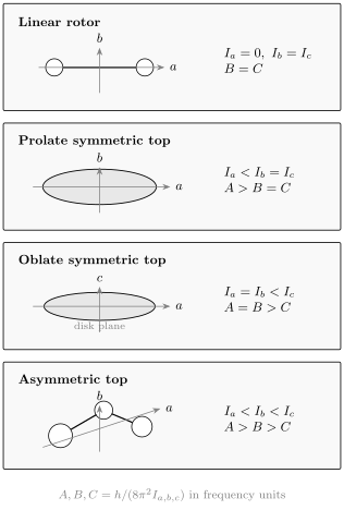
Rigid-rotor classes are statements about principal moments of inertia. Because each rotational constant is inversely proportional to its moment, the inequalities reverse between $I_a,I_b,I_c$ and $A,B,C$. Molecular examples can carry inversion, internal-rotation, spin, or vibronic structure beyond the shapes shown.

Linear and spherical tops

A linear rotor has

$$I_a=0, \qquad I_b=I_c,$$

and only the two perpendicular rotations produce the scalar ladder $E_J\propto J(J+1)$.

A spherical top has

$$I_a=I_b=I_c, \qquad A=B=C.$$

Its rotational Hamiltonian is also proportional to $\hat J^2$, but the configuration space is the full orientation of a three-dimensional body rather than only a molecular axis. Methane and sulfur hexafluoride are standard high-symmetry examples, although their ordinary pure rotational electric-dipole spectra vanish in the rigid equilibrium limit because they have no permanent dipole.

Symmetric tops

A prolate symmetric top has

$$I_a<I_b=I_c, \qquad A>B=C,$$

while an oblate symmetric top has

$$I_a=I_b<I_c, \qquad A=B>C.$$

Let $B_\parallel$ be the constant for the symmetry axis and $B_\perp$ the common perpendicular constant. Then

$$\frac{E_{J,K}}{h} = B_\perp J(J+1) + (B_\parallel-B_\perp)K^2,$$

with

$$J=0,1,2,\ldots, \qquad K=-J,\ldots,J.$$

For a prolate top, $B_\parallel=A$; for an oblate top, $B_\parallel=C$. In a field-free rigid symmetric top the energy depends on $K^2$, so $K$ and $-K$ are degenerate before additional interactions are included.

Asymmetric tops

Most polyatomic molecules satisfy

$$I_a<I_b<I_c, \qquad A>B>C.$$

Because no body-axis projection commutes with the full asymmetric-top Hamiltonian, there is no exact $K$ quantum number and no universal closed-form energy formula. For each $J$, one constructs and diagonalizes a finite matrix in a symmetric-top basis.

Ray’s asymmetry parameter is

$$\kappa = \frac{2B-A-C}{A-C}, \qquad -1\le\kappa\le1.$$

The prolate symmetric-top limit is $\kappa=-1$ and the oblate limit is $\kappa=+1$. The conventional labels

$$J_{K_a,K_c}$$

record correlation with those two limits. They are useful labels, not simultaneous exact projections of $\mathbf J$ on two body axes.

For semirigid asymmetric tops, precision work usually adds quartic and then sextic centrifugal-distortion operators. Watson’s reduced Hamiltonians remove parameter indeterminacies, but different reductions and axis representations produce different numerical parameter sets. Constants should therefore be compared only after matching conventions.

Microwave Spectroscopy Connection

What is measured

Microwave, millimeter-wave, and submillimeter spectroscopy measures electromagnetic frequencies associated with transitions. In absorption one records attenuation; in Fourier-transform microwave methods, a pulse prepares rotational coherence and the emitted free-induction decay is Fourier transformed.

The basic inference chain is

$$\begin{gathered} \text{measured frequencies}\\ \Downarrow\\ \text{assigned quantum-number transitions}\\ \Downarrow\\ \text{effective-Hamiltonian fit}\\ \Downarrow\\ \text{rotational and coupling constants}\\ \Downarrow\\ \text{moments, structure, and predictions}. \end{gathered}$$

Every arrow introduces assumptions. Assignment uses predicted patterns and selection rules. Fitting chooses a Hamiltonian and weighting model. Structural inference chooses a vibrational correction and geometry model.

Positions, strengths, and populations

Line positions come from energy differences:

$$h\nu_{fi}=E_f-E_i.$$

Integrated strengths also depend on the transition moment and lower-state population. For an ideal linear rotor in thermal equilibrium,

$$N_J \propto g_{\mathrm{ns}}(J) (2J+1) \exp\left[ -\frac{E_J}{k_BT} \right],$$

where $g_{\mathrm{ns}}(J)$ is the nuclear-spin statistical weight. Ignoring that factor and treating $J$ as continuous, the most populated region is near

$$J_{\mathrm{peak}} \approx \sqrt{ \frac{k_BT} {2hc\widetilde B} } -\frac{1}{2}.$$

This estimate predicts where intensity may concentrate, not the intensity of an individual line. Dipole components, Hönl–London factors, stimulated emission, partition functions, instrumental response, optical depth, collisions, and nonequilibrium populations can all matter.

What different patterns constrain

Spectroscopic evidence	Primary constraint
Line spacings and assignments	$A,B,C$ and distortion constants
Isotopologue shifts	mass distribution and structural coordinates
Stark shifts	body-fixed dipole components
Hyperfine splittings	nuclear quadrupole, spin-rotation, and spin-spin couplings
Relative intensities	populations, dipole components, and line-strength factors
Residual trends	missing distortion, coupling, perturbation, or misassignment

A rotational spectrum is often a distinctive molecular fingerprint because different isomers and isotopologues have different inertia tensors. Enantiomers in an isolated achiral environment, however, have the same ordinary rotational constants. Additional chiral discrimination requires a chiral interaction or phase-sensitive multi-axis protocol.

A defensible fitting workflow

1. State the isotopologue, electronic state, vibrational state, and angular-momentum coupling convention.
2. Predict low-order patterns from estimated $A,B,C$, dipole components, and selection rules.
3. Assign connected transitions rather than isolated lines.
4. Fit the smallest effective Hamiltonian supported by the measured range and uncertainties.
5. Inspect signed residuals against $J$, $K_a$, $K_c$, frequency, and experimental subset.
6. Add distortion or coupling terms only when residual structure and parameter significance justify them.
7. Propagate the covariance matrix when predicting unmeasured lines.
8. Validate with isotopologues, combination differences, independent frequency bands, or ab initio constants.
9. Report the Hamiltonian reduction, axis representation, units, parameter correlations, and measured range.
10. Do not extrapolate a truncated effective Hamiltonian through a resonance or toward dissociation.

Curated catalogs such as the JPL Molecular Spectroscopy Catalog and the Cologne Database for Molecular Spectroscopy distribute frequencies, uncertainties, intensities, assignments, and documentation. A catalog entry is a model-based evaluation of laboratory data, not a replacement for the cited primary measurements or the entry documentation.

Approximation Hierarchy

A useful hierarchy for molecular rotation is:

$$\begin{gathered} \text{rigid rotor}\\ \subset\\ \text{semirigid rotor with distortion}\\ \subset\\ \text{rovibrational effective Hamiltonian}\\ \subset\\ \text{coupled rovibronic and spin model}\\ \subset\\ \text{full nuclear motion on coupled surfaces}. \end{gathered}$$

Move upward when the data require it. Typical warning signs are:

• residuals that grow systematically with $J$ or $K$;
• perturbations localized near a level crossing;
• tunneling or internal-rotation splittings;
• strong Coriolis, $\ell$-type, spin-orbit, or vibronic coupling;
• large-amplitude motion for which one equilibrium frame is inadequate;
• rotational excitation approaching a barrier or dissociation threshold.

More parameters do not automatically mean a more physical model. An effective Hamiltonian can interpolate measured lines very accurately while its individual high-order constants are strongly correlated or convention dependent.

Common Mistakes

• Treating $B_e$, $B_0$, and $B_v$ as interchangeable. They correspond to different nuclear-motion averages.
• Mixing energy, hertz, and wavenumber constants without factors of $h$ or $c$.
• Calling a fitted ground-state distance an equilibrium bond length.
• Inferring a unique polyatomic geometry from only three constants of one isotopologue.
• Saying a nonpolar molecule has no rotational levels. It lacks the leading electric-dipole pure rotational probe.
• Deriving a selection rule from level spacing rather than from a transition matrix element.
• Using $J$ where an open-shell convention uses $N$, or ignoring coupled spin labels.
• Treating $K_a$ and $K_c$ as simultaneous exact projections for an asymmetric top.
• Comparing Watson-Hamiltonian constants from different reductions as if their numerical values were invariant.
• Assuming every high-$J$ deviation is centrifugal distortion. Resonances, misassignments, calibration errors, and unresolved structure can produce trends.
• Extrapolating a polynomial effective Hamiltonian far outside its fitted quantum-number and frequency range.
• Reading line intensity as population alone. Matrix elements and experimental transfer functions also matter.

Exercises

1. Inertia and an effective bond length

A closed-shell diatomic has $B_0=57.64\,\mathrm{GHz}$ and reduced mass $\mu=6.856\,\mathrm u$. Estimate $I_0$ and $R_0$. Use $1\,\mathrm u=1.66054\times10^{-27}\,\mathrm{kg}$.

Solution

In frequency units,

$$I_0 = \frac{h}{8\pi^2B_0}.$$

With $B_0=5.764\times10^{10}\,\mathrm{s^{-1}}$,

$$I_0 \approx 1.46\times10^{-46}\,\mathrm{kg\,m^2}.$$

The reduced mass is

$$\begin{aligned} \mu &= 6.856(1.66054\times10^{-27}),\\ &\approx 1.139\times10^{-26}\,\mathrm{kg}. \end{aligned}$$

Therefore

$$\begin{aligned} R_0 &= \sqrt{\frac{I_0}{\mu}}\\ &\approx 1.13\times10^{-10}\,\mathrm m\\ &= 1.13\,\text{\AA}. \end{aligned}$$

Because the input is $B_0$, this is an effective ground-state distance $R_0$, not automatically $R_e$.

2. Diatomic isotope scaling

Approximate the masses of $^{12}\mathrm C$, $^{13}\mathrm C$, and $^{16}\mathrm O$ by their mass numbers. If the bond length is unchanged, estimate $B(^{13}\mathrm C{}^{16}\mathrm O)/B(^{12}\mathrm C{}^{16}\mathrm O)$.

Solution

The reduced masses are

$$\mu_{12,16} = \frac{12(16)}{12+16} = \frac{48}{7}\,\mathrm u$$

and

$$\mu_{13,16} = \frac{13(16)}{13+16} = \frac{208}{29}\,\mathrm u.$$

Since $B\propto1/\mu$ at fixed distance,

$$\begin{aligned} \frac{B_{13,16}}{B_{12,16}} &= \frac{\mu_{12,16}}{\mu_{13,16}}\\ &\approx 0.956. \end{aligned}$$

The heavier isotopologue has the smaller rotational constant and more closely spaced lines.

3. Distorted HCN line

Using $B_0=44\,315.9757\,\mathrm{MHz}$ and $D_0=0.08724\,\mathrm{MHz}$, calculate the HCN $J=2\rightarrow3$ centroid frequency through quartic distortion.

Solution

For $J\rightarrow J+1$,

$$\nu = 2B_0(J+1) -4D_0(J+1)^3.$$

At $J=2$,

$$\begin{aligned} \nu &= 6B_0-108D_0\\ &= 265\,895.8542\,\mathrm{MHz} -9.42192\,\mathrm{MHz}\\ &= 265\,886.4323\,\mathrm{MHz}. \end{aligned}$$

This is a rotational centroid within the truncated model. Nitrogen quadrupole coupling splits an actual high-resolution feature into hyperfine components.

4. Sign of centrifugal distortion

Starting from

$$\begin{aligned} E(x) &= \frac{1}{2}kx^2 + \frac{\hbar^2K}{2\mu(R_e+x)^2},\\ K &= J(J+1), \end{aligned}$$

show that the leading correction to $B_EK$ is negative.

Solution

Expand to first order in $x$ when finding the minimum:

$$\frac{dE}{dx} \approx kx -\frac{\hbar^2K}{\mu R_e^3}.$$

Thus

$$x_J \approx \frac{\hbar^2K}{\mu kR_e^3}.$$

Keeping terms through $K^2$ after substitution gives

$$E_J \approx \frac{\hbar^2K}{2\mu R_e^2} - \frac{\hbar^4K^2}{2\mu^2kR_e^6}.$$

Therefore

$$E_J=B_EK-D_EK^2, \qquad D_E>0.$$

Stretching increases the moment of inertia, so high-$J$ energies lie below the rigid-rotor prediction.

5. Classify a rotor

A molecule has principal moments in the ratio

$$I_a:I_b:I_c=3:12:12.$$

Classify the rotor and find the ratio $A:B:C$.

Solution

Because

$$I_a<I_b=I_c,$$

the molecule is a prolate symmetric top. Rotational constants are inversely proportional to moments:

$$A:B:C = \frac{1}{3}:\frac{1}{12}:\frac{1}{12} = 4:1:1.$$

6. Identify an asymmetric-top transition type

Classify each transition by its $a$-, $b$-, or $c$-type parity rule:

$$2_{12}\rightarrow1_{01}, \qquad 2_{02}\rightarrow1_{01}.$$

Solution

For

$$2_{12}\rightarrow1_{01},$$

both changes are odd:

$$\Delta K_a=-1, \qquad \Delta K_c=-1.$$

It is therefore $b$ type.

For

$$2_{02}\rightarrow1_{01},$$

the changes are

$$\Delta K_a=0, \qquad \Delta K_c=-1.$$

Even $\Delta K_a$ and odd $\Delta K_c$ identify an $a$-type transition.

7. Thermal rotational population

For a linear rotor with $\widetilde B=2.00\,\mathrm{cm}^{-1}$ at $T=100\,\mathrm K$, estimate the most populated $J$, ignoring nuclear-spin weights. Use $k_B/(hc)=0.6950\,\mathrm{cm^{-1}\,K^{-1}}$.

Solution

The continuous estimate is

$$J_{\mathrm{peak}} \approx \sqrt{ \frac{k_BT} {2hc\widetilde B} } -\frac{1}{2}.$$

Since

$$\frac{k_BT}{hc} = 69.50\,\mathrm{cm}^{-1},$$

we find

$$\begin{aligned} J_{\mathrm{peak}} &\approx \sqrt{\frac{69.50}{4.00}} -\frac{1}{2}\\ &\approx 3.67. \end{aligned}$$

The nearest integer is $J=4$. Exact discrete populations should be compared at $J=3$ and $J=4$, and observed line intensity still requires a transition-strength factor.

8. Precision versus structural meaning

An asymmetric-top fit determines $A_0,B_0,C_0$ to relative precision $10^{-8}$. Explain why this does not establish every equilibrium bond length and angle to relative precision $10^{-8}$.

Solution

The fitted constants determine three ground-state principal moments with high precision. A polyatomic geometry has more than three internal coordinates, so one isotopologue does not make the inverse problem unique. Moreover, $A_0,B_0,C_0$ include zero-point vibrational averaging, while an equilibrium structure refers to the potential minimum.

Recovering $r_e$ requires additional information such as multiple isotopologues, structural constraints, and calculated rotation–vibration corrections. Frequency precision, effective-Hamiltonian precision, and structural accuracy are distinct quantities.

Key Takeaways

• Molecular rotation is an effective description of nuclear reorientation after translation and internal shape motion are separated.
• Rotational constants are inverse moments of inertia, but their numerical meaning depends on energy, frequency, or wavenumber units.
• $B_e$, $B_v$, and $B_0$ describe different levels of vibrational averaging.
• Electric-dipole selection rules belong to transition matrix elements; nonpolar molecules still possess rotational states.
• Positive centrifugal distortion lowers high-$J$ levels relative to the rigid ladder and limits extrapolation.
• Symmetric tops have an exact body-axis projection $K$; asymmetric tops use limiting labels $K_a,K_c$ and require matrix diagonalization.
• Microwave frequencies constrain effective Hamiltonians directly. Geometry, dipoles, and dynamics follow through additional models and measurements.

Cross-Links

• Common Molecular Hamiltonians compares rigid, rovibrational, electronic spin–rotation, and nuclear hyperfine operator conventions.
• Molecular Quantum Mechanics places rotation in the electronic–vibrational–rotational energy hierarchy.
• Molecular Hamiltonian derives the laboratory and internal many-particle Hamiltonians.
• Born–Oppenheimer in Molecules explains the one-surface nuclear Hamiltonian and rotation–vibration separation.
• Potential Energy Surfaces defines equilibrium geometries, curvatures, barriers, and dissociation limits.
• Vibrations of Diatomics develops bond-stretch term values, isotope scaling, anharmonicity, and the vibrational origins around which gas-phase rotational branches are organized.
• Rovibrational Coupling combines rotational and vibrational term values into branch-resolved spectra and develops their leading interaction corrections.
• Rotational Spectroscopy develops experimental line assignment, isotope comparison, evaluated-catalog use, and structure-inference cautions.
• Precision Molecular Measurements uses parity-doublet orientation and rotational Stark response as calibrated resources for electron, nuclear, and chiral symmetry probes.
• Rigid Rotor is the canonical derivation of $J(J+1)$ levels and spherical-harmonic eigenfunctions.
• Rotational Spectra gives the first ideal line-ladder calculation.
• Applications to Molecular Rotations derives electric-dipole rules with irreducible tensors and three-j symbols.
• Molecular Physics Applications organizes rotational, vibrational, point-group, and field-response symmetry.
• Wigner D-Matrices provide the natural orientation basis for symmetric and asymmetric tops.
• Selection Rules and Transition Rates separates symmetry zeros, matrix elements, and rates.
• Quantum Chemistry Roadmap places molecular rotation in a broader study sequence.
• Quantum Chemistry References provides a wider source ladder for molecular structure and spectroscopy.

References

• J. M. Brown and A. Carrington, Rotational Spectroscopy of Diatomic Molecules, Cambridge University Press, 2003.
• P. R. Bunker and P. Jensen, Molecular Symmetry and Spectroscopy, 2nd ed., NRC Research Press, 1998.
• P. F. Bernath, Spectra of Atoms and Molecules, 4th ed., Oxford University Press, 2025.
• C. H. Townes and A. L. Schawlow, Microwave Spectroscopy, McGraw–Hill, 1955; Dover reprint, 1975.
• W. Gordy and R. L. Cook, Microwave Molecular Spectra, 3rd ed., Wiley, 1984.
• R. N. Zare, Angular Momentum: Understanding Spatial Aspects in Chemistry and Physics, Wiley, 1988.
• E. B. Wilson Jr., J. C. Decius, and P. C. Cross, Molecular Vibrations, McGraw–Hill, 1955; Dover reprint, 1980.
• J. K. G. Watson, “Determination of Centrifugal Distortion Coefficients of Asymmetric-Top Molecules,” Journal of Chemical Physics 46, 1935–1949 (1967), doi:10.1063/1.1840957.
• J. K. G. Watson, “Simplification of the Molecular Vibration-Rotation Hamiltonian,” Molecular Physics 15, 479–490 (1968), doi:10.1080/00268976800101381.
• J. Kraitchman, “Determination of Molecular Structure from Microwave Spectroscopic Data,” American Journal of Physics 21, 17–24 (1953), doi:10.1119/1.1933338.
• C. C. Costain, “Determination of Molecular Structures from Ground State Rotational Constants,” Journal of Chemical Physics 29, 864–874 (1958), doi:10.1063/1.1744602.
• NIST Physical Measurement Laboratory, Triatomic Spectral Database: molecular parameters and energy-level formulation and evaluated HCN isotopologue constants.
• H. M. Pickett, R. L. Poynter, E. A. Cohen, M. L. Delitsky, J. C. Pearson, and H. S. P. Müller, “Submillimeter, Millimeter, and Microwave Spectral Line Catalog,” Journal of Quantitative Spectroscopy and Radiative Transfer 60, 883–890 (1998), doi:10.1016/S0022-4073(98)00091-0.
• C. P. Endres, S. Schlemmer, P. Schilke, J. Stutzki, and H. S. P. Müller, “The Cologne Database for Molecular Spectroscopy, CDMS, in the Virtual Atomic and Molecular Data Centre, VAMDC,” Journal of Molecular Spectroscopy 327, 95–104 (2016), doi:10.1016/j.jms.2016.03.005.