Conical Intersections

A conical intersection is a nuclear geometry at which two adiabatic electronic energies are exactly degenerate and split linearly in two independent nuclear directions. In the two-dimensional plane that lifts the degeneracy, the local energy sheets have the topology of a double cone. In the full molecular coordinate space, the degeneracies usually form a high-dimensional intersection seam, not one isolated point.

Conical intersections are central because they unite three ideas that are easy to confuse:

• an exact degeneracy in an electronic eigenvalue problem;
• strong coupling of electronic and nuclear motion near that degeneracy;
• nontrivial phase acquired by adiabatic transport around the degeneracy.

These are related, but they are not identical. A wavepacket can pass through a coupling region and change electronic surface without completing a loop. A loop can acquire a geometric phase while remaining gapped and approximately adiabatic. An optimized crossing geometry can exist yet be dynamically inaccessible from a specified preparation.

The defining equality is simple,

$$E_1(R_{\mathrm{CI}}) = E_2(R_{\mathrm{CI}}),$$

but a useful description must also identify the electronic-state manifold, spin and symmetry assumptions, branching directions, seam coordinates, energetic accessibility, nuclear dynamics, and observable.

Canonical Scope

This page is the canonical molecular home for:

• degeneracy conditions for two real electronic states;
• codimension-two seam counting in polyatomic molecules;
• the gradient-difference and interstate-coupling vectors;
• the local branching-plane Hamiltonian and double-cone topology;
• minimum-energy conical intersections and seam topography;
• the distinction between crossing geometry and nonadiabatic dynamics;
• molecular Berry phase around a conical intersection;
• photochemical pathway logic and computational validation.

Potential Energy Surfaces owns general molecular landscape geometry and uncertainty. Nonadiabatic Coupling owns the exact channel-coupling handoff, wavepacket branching, surface hopping, vibronic models, and dynamics-method caveats. Born–Oppenheimer Berry Phase owns the broader gauge and holonomy construction. This page concentrates those ingredients on the geometry and consequences of an electronic degeneracy.

Degeneracies in Molecular Potential Surfaces

A two-state degeneracy requires two conditions

Near an isolated pair of states, choose a real electronic basis and write the effective electronic Hamiltonian as

$$\mathbf W(R) = \begin{pmatrix} W_{11}(R) & W_{12}(R) \\ W_{12}(R) & W_{22}(R) \end{pmatrix}.$$

Its two eigenvalues are equal exactly when the traceless part vanishes:

$$\begin{aligned} W_{11}(R)-W_{22}(R)&=0, \\ W_{12}(R)&=0. \end{aligned}$$

These are two independent scalar conditions. A generic double degeneracy of a real symmetric Hamiltonian therefore has codimension two. This is the molecular form of the von Neumann–Wigner counting rule.

The assumptions matter. The usual count applies to two states of the same spin in a spin-free, time-reversal-invariant problem for which a real representation can be chosen. A general complex Hermitian two-state Hamiltonian has a third Pauli-matrix component, so a generic degeneracy has codimension three. Spin–orbit coupling, magnetic fields, Kramers structure, and additional exact symmetries require their own count.

Why a seam is more common than a point

Let $F$ be the number of independent internal nuclear coordinates. Imposing two degeneracy conditions leaves a seam of generic dimension

$$\dim\mathcal S = F-2.$$

For a nonlinear molecule with $N_N$ nuclei,

$$\begin{aligned} F&=3N_N-6, \\ \dim\mathcal S&=3N_N-8. \end{aligned}$$

Thus a nonlinear triatomic molecule has a one-dimensional seam in its complete three-dimensional internal coordinate space. A two-coordinate plot intersects that seam at a point and displays the familiar cone. A larger polyatomic molecule can possess an extensive family of degenerate geometries with different energies, structures, and dynamical consequences.

A diatomic molecule has only one internal coordinate, so two same-symmetry states do not generically form an accidental conical intersection as the bond length alone changes. Curves of different exact symmetry can cross because symmetry forces their coupling to vanish, but that is a different counting problem.

Linear geometries also need special care. Their vibrational-coordinate count differs from the nonlinear count, and bending degeneracies can produce Renner–Teller structure. One should not insert $3N_N-8$ mechanically at a linear configuration.

Accidental and symmetry-associated intersections

“Accidental” does not mean physically unlikely. It means that no named point-group symmetry forces the equality. Because a polyatomic molecule supplies many coordinates, satisfying two independent conditions is generic enough to produce extended seams.

Symmetry can still organize an intersection:

• two states in different irreducible representations may cross within a symmetry-preserving subspace because their coupling vanishes there;
• a symmetry-breaking coordinate can become the coupling direction and open the gap;
• an electronically degenerate state at a high-symmetry geometry can undergo Jahn–Teller splitting;
• lowering symmetry can turn a protected crossing into an avoided crossing.

The labels “symmetry-allowed crossing,” “Jahn–Teller intersection,” and “accidental same-symmetry conical intersection” should not be treated as synonyms. Their local Hamiltonians may look similar after reduction, but their global seam structure and allowed perturbations differ.

Same spin is not different spin

A conical intersection usually refers to two adiabatic states in the same spin manifold when spin–orbit coupling is neglected. A singlet and a triplet can cross on a codimension-one seam in that spin-free model because their electronic coupling is zero by spin symmetry. Once spin–orbit coupling is included, the relevant spin-mixed states can repel and the dynamics becomes an intersystem-crossing problem.

The practical report must therefore say which states intersect, their multiplicities, whether spin–orbit coupling is included, and which symmetry constraints were imposed.

Geometry of Conical Intersections

The branching-plane vectors

Let $R_{\mathrm{CI}}$ be a point on a two-state seam and let

$$q=R-R_{\mathrm{CI}}$$

denote a small displacement in internal, mass-weighted, or otherwise declared nuclear coordinates. For real adiabatic states, define the gradient-difference vector

$$\mathbf g = \frac{1}{2} \left[ \nabla_R E_2- \nabla_R E_1 \right]_{R_{\mathrm{CI}}}$$

and the interstate-coupling vector

$$\mathbf h = \left[ \langle\phi_1| \nabla_R H_e |\phi_2\rangle \right]_{R_{\mathrm{CI}}}.$$

The two-dimensional subspace

$$\mathcal B = \operatorname{span} \{\mathbf g,\mathbf h\}$$

is the branching plane. Displacements in this plane lift the degeneracy to first order. Directions orthogonal to both vectors are tangent, to first order, to the intersection seam.

The vector $\mathbf h$ is finite in a well-defined two-state diabatic description. It should not be confused with the adiabatic derivative coupling

$$\mathbf d_{12} = \langle\phi_1|\nabla_R\phi_2\rangle,$$

which away from degeneracy obeys

$$\mathbf d_{12} = \frac{ \langle\phi_1|\nabla_R H_e|\phi_2\rangle }{E_2-E_1}$$

and is generically singular as the adiabatic gap closes. At the degeneracy itself, the individual adiabatic eigenvectors are not unique, so a reported derivative-coupling vector requires a limiting convention or a smooth electronic subspace construction.

Local two-state normal form

After a rotation within the two-state electronic subspace, the first-order Hamiltonian can be written

$$\begin{aligned} H_{\mathrm{eff}}(q) ={}& \left[ E_{\mathrm{CI}}+ \mathbf s\cdot q \right]\mathbf 1 \\ &+ (\mathbf g\cdot q)\sigma_z \\ &+ (\mathbf h\cdot q)\sigma_x +O(q^2). \end{aligned}$$

The vector $\mathbf s$ is the average-energy gradient at the seam point. It tilts both sheets together. The eigenvalues are

$$\begin{aligned} E_\pm(q) ={}&E_{\mathrm{CI}} +\mathbf s\cdot q \\ &\pm \sqrt{ (\mathbf g\cdot q)^2 + (\mathbf h\cdot q)^2 } +O(q^2). \end{aligned}$$

Choose orthogonal branching coordinates $x$ and $y$ so that the two gap-opening terms become $\kappa_x x$ and $\kappa_y y$. Then

$$E_+(x,y)-E_-(x,y) = 2\sqrt{ \kappa_x^2x^2+ \kappa_y^2y^2 }.$$

The gap is linear in radial displacement from the seam. If $\kappa_x\ne\kappa_y$, the cone is elliptic rather than circular. Higher-order terms curve and warp both the cone and the seam.

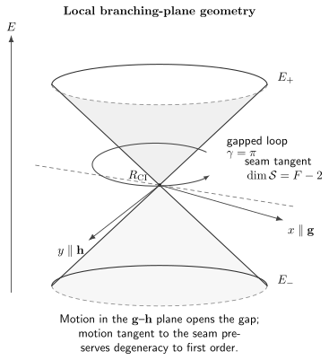
At one point of an intersection seam, the gradient-difference direction $\mathbf g$ and interstate-coupling direction $\mathbf h$ span the branching plane. Motion in either direction opens the adiabatic gap linearly; motion tangent to the $(F-2)$-dimensional seam preserves degeneracy to first order. A gapped loop around the seam carries the molecular geometric phase.

A cone is a local statement

The double cone is the first-order energy splitting in the branching plane. It does not assert that the entire molecular surface is cone-shaped. Beyond a sufficiently small neighborhood:

• the seam bends through nuclear coordinate space;
• the average energy changes along the seam;
• branching directions rotate;
• other electronic states can enter;
• quadratic and higher vibronic couplings can change the topography;
• dissociation coordinates and environmental coordinates can alter accessibility.

The words peaked and sloped describe how the common tilt competes with the gap-opening slopes near an appropriate seam critical point. They are useful local classifications, not complete predictors of a quantum yield.

Minimum-energy conical intersections

A minimum-energy conical intersection (MECI) is a local minimum of a chosen seam energy subject to the degeneracy constraint. With

$$\bar E(R) = \frac{E_1(R)+E_2(R)}{2},$$

the idealized problem is

$$\begin{gathered} \underset{R}{\operatorname{minimize}} \quad \bar E(R), \\ \text{subject to} \quad E_2(R)-E_1(R)=0. \end{gathered}$$

An MECI is analogous to a stationary landmark on the crossing seam, but it is not automatically a transition state and not necessarily the seam point reached by a wavepacket. A dynamically important point may instead minimize distance from a Franck–Condon geometry, lie on a constrained reaction coordinate, or occur where the incoming wavepacket has substantial amplitude and favorable momentum.

Different optimizations can find different local MECIs on the same connected seam or on disconnected seams. Reporting “the conical intersection” without a state pair, geometry, energy reference, optimization objective, and electronic-structure model is therefore incomplete.

Why a one-dimensional scan shows an avoided crossing

Take a straight cut through the local cone but miss the seam by a fixed offset $b$ in the second branching coordinate:

$$\begin{aligned} x&=q, \\ y&=b. \end{aligned}$$

Along that cut,

$$\begin{aligned} \Delta E(q) ={}&2\sqrt{ \kappa_x^2q^2+ \kappa_y^2b^2 }, \\ \Delta E_{min} ={}&2|\kappa_yb|. \end{aligned}$$

Only the cut with $b=0$ reaches the exact degeneracy. This is why a one-dimensional reaction-coordinate plot often displays an avoided crossing even when the full multidimensional molecular problem contains a conical-intersection seam.

Nonadiabatic Transitions

The adiabatic basis fails at the apex

The adiabatic electronic eigenvectors are defined only up to phase away from degeneracy and up to an arbitrary unitary rotation inside a degenerate subspace at the seam. As the gap closes, trying to track two separate adiabatic states produces rapidly varying eigenvectors and singular derivative couplings.

That singularity is not an infinite physical force. It signals that the one-surface adiabatic representation has become a poor coordinate system for the coupled electron–nuclear state. A smooth diabatic or quasi-diabatic two-state subspace can keep the Hamiltonian matrix finite while moving the coupling into off-diagonal potential terms.

Passage creates branching, not a universal jump

An excited nuclear wavepacket approaching a conical-intersection region can:

• remain partly on the upper adiabatic sheet;
• transfer amplitude to the lower sheet;
• split into branches with different nuclear momenta;
• acquire relative phase and later interfere;
• miss the seam but still undergo substantial transfer in a small-gap region;
• encounter another state before the two-state event is complete.

There is no state-independent “transition probability of the conical intersection.” The result depends on the incoming nuclear wavepacket, its direction and momentum in the branching plane, the local tilt and anisotropy, seam-coordinate motion, electronic coherence, additional states, and the measured observable.

The same warning applies to the funnel metaphor. A low and accessible crossing region can support rapid internal conversion, but an intersection is not a drain that captures every trajectory or transfers all population.

Relation to Landau–Zener passage

A prescribed one-dimensional path through or near the branching plane can sometimes be reduced locally to a Landau–Zener-like sweep. That model can illuminate gap and speed dependence. It does not represent the full multidimensional wavepacket automatically:

• the second branching coordinate controls whether the path hits or misses the seam;
• nuclear momentum can rotate and branch;
• repeated passages create interference;
• the adiabatic state labels exchange character around the cone;
• the wavepacket samples a distribution of paths rather than one classical sweep.

Landau–Zener Transition owns the exactly solvable sweep. Nonadiabatic Coupling compares wavepacket, spawning, mean-field, surface-hopping, and perturbative dynamics methods.

Method choice follows the observable

Full quantum propagation on a reduced vibronic Hamiltonian can retain branching, tunneling, coherence, and geometric-phase interference. Gaussian spawning methods expand the nuclear state adaptively near branching regions. Surface hopping samples active-surface histories but requires explicit conventions for state tracking, decoherence, frustrated hops, and momentum adjustment. Mean-field dynamics can retain electronic coherence but may average forces across distinct products.

No method becomes reliable merely because it reaches a small computed gap. The electronic states, initial ensemble, nuclear coordinates, timestep, energy conservation, state populations, and asymptotic products must all be validated.

Berry Phase in Molecules

Half-angle structure of a two-state eigenvector

For a circularized branching plane, write

$$\begin{aligned} x&=\rho\cos\varphi, \\ y&=\rho\sin\varphi, \end{aligned}$$

and omit the common energy and tilt. The local electronic Hamiltonian becomes

$$H'(\rho,\varphi) = \kappa\rho \left( \cos\varphi\,\sigma_z + \sin\varphi\,\sigma_x \right).$$

One real normalized lower-state eigenvector can be chosen as

$$|\phi_-(\varphi)\rangle = \begin{pmatrix} -\sin(\varphi/2) \\ \cos(\varphi/2) \end{pmatrix}.$$

After one circuit,

$$|\phi_-(\varphi+2\pi)\rangle = -|\phi_-(\varphi)\rangle.$$

The sign of one eigenvector at one geometry is a gauge choice. The impossibility of choosing a globally single-valued real eigenvector around a loop that encloses the seam is the invariant content. In a complex gauge, the same holonomy appears as a Berry phase

$$\gamma=\pi \pmod{2\pi}.$$

The total molecular state remains single-valued

In a one-surface adiabatic product,

$$\Psi(r,R) = \phi_-(r;R)\chi_-(R),$$

the electronic sign change must be compensated by the nuclear factor, or equivalently by including the Mead–Truhlar vector potential in the nuclear Hamiltonian. The geometric phase can then alter nodal structure, level patterns, interference between paths, and reaction amplitudes.

This phase is not an electronic transition. The loop used to define it stays in a region where the chosen electronic state is gapped. Dynamics through the seam and adiabatic transport around the seam are distinct limits of the same geometry-dependent electronic subspace.

When the simple π rule needs refinement

The elementary sign-change result assumes an isolated real two-state conical intersection and a loop linked once with the relevant seam. More generally:

• a loop can enclose several intersections whose phase factors combine;
• the electronic subspace can contain more than two important states;
• spin–orbit coupling can require a complex, possibly non-Abelian connection;
• the seam can curve and reconnect globally;
• exact electron–nuclear factorization changes how the phase is partitioned between factors.

The physical question is always about loop, subspace, gauge-covariant holonomy, and observable. Born–Oppenheimer Berry Phase develops that structure in full.

Photochemical Significance

A four-stage pathway

A common photochemical sequence is:

1. Preparation. Absorption creates a nuclear wavepacket on one or more electronically excited states in a Franck–Condon region.
2. Approach. Excited-state forces carry some amplitude toward an accessible small-gap or conical-intersection region.
3. Transfer. Electronic and nuclear amplitudes mix, often producing internal conversion to a lower state.
4. Branching. The outgoing lower-state wavepacket evolves toward reactants, isomers, fragments, or other products.

This sequence explains why excited-state chemistry cannot usually be inferred from a vertical excitation energy alone. The gradients and couplings between the preparation region and the seam, not only the MECI energy, control accessibility.

Product selectivity is dynamical

The gradient-difference direction tends to distinguish the two local adiabatic sheets, while the coupling direction mixes electronic character. Incoming momentum and the lower-surface slopes can steer different pieces of the wavepacket toward different products. Seam-coordinate motion adds many more approach and exit channels.

Consequently, a static conical-intersection geometry can suggest candidate coordinates but cannot by itself determine a branching ratio. Product yields are asymptotic observables requiring propagation, ensemble sampling, or an experimentally constrained kinetic model.

Internal conversion and photostability

Conical intersections can provide efficient radiationless return from an excited singlet to a lower singlet. Such pathways are implicated in photoisomerization and ring opening, and they can contribute to rapid deactivation of some nucleobases and amino-acid chromophores. The careful claim is can contribute: solvent, protonation, substitution, competing states, barriers, spin–orbit coupling, and initial excitation conditions can all redirect the dynamics.

Internal conversion should not be confused with fluorescence, phosphorescence, or intersystem crossing. A realistic photochemical model may require all of them, with rates or explicit dynamics matched to the relevant time and energy scales.

Conical intersections are not ordinary transition states

A ground-state transition state is a saddle of one potential-energy surface used in a statistical reaction-rate construction. A conical intersection is a degeneracy between electronic surfaces. Both can organize reaction pathways, but their mathematics and dynamics differ:

• a transition state is characterized by curvature on one surface;
• a conical intersection is characterized by a seam and two gap-opening directions;
• passage near a conical intersection involves electronic-state mixing and coherence;
• recrossing, branching, and geometric phase may be essential.

Calling an MECI the “transition state of photochemistry” can be a useful analogy only when these differences remain explicit.

Computational Challenges

Electronic states must be balanced

Near degeneracy, a method must describe both states with comparable orbital, correlation, and state-averaging errors. A small unbalanced error can move the seam, rotate the branching plane, change its energy, or open a spurious gap.

State-averaged CASSCF often gives the correct qualitative multireference topology and analytic derivative couplings, but its result depends on active space, orbital optimization, state weights, and omitted dynamic correlation. Multireference configuration interaction and multistate perturbation methods can add correlation at greater cost and with their own intruder-state and invariance issues.

Ordinary single-reference methods can become ill-conditioned as reference character changes. Conventional linear-response TDDFT does not generally provide the correct topology for a ground-state/excited-state conical intersection; spin-flip and ensemble approaches repair some cases but introduce method-specific assumptions. A method label is therefore not a validation argument.

Electronic Structure Overview owns the broader hierarchy of basis-set, correlation, multireference, and excited-state errors.

Locating a seam point

A conical-intersection optimizer must reduce the energy gap while minimizing the average energy along the seam. If orthonormal vectors $\widehat{\mathbf g}$ and $\widehat{\mathbf h}$ span the branching plane, the first-order projector into the seam tangent space is

$$\mathbf P_{\mathcal S} = \mathbf 1 - \widehat{\mathbf g} \widehat{\mathbf g}^{\mathsf T} - \widehat{\mathbf h} \widehat{\mathbf h}^{\mathsf T}.$$

The projected average-energy gradient

$$\mathbf P_{\mathcal S} \nabla_R\bar E$$

drives motion along the seam, while separate gap-closing components drive the geometry toward degeneracy. Direct gradient-projection algorithms, constrained optimization, sequential penalty methods, and branching-plane-update methods implement this logic in different ways.

When derivative couplings are unavailable, a penalty objective such as

$$F_\mu(R) = \bar E(R) + \mu[\Delta E(R)]^2$$

can be used sequentially or combined with approximate branching-space information. A finite penalty alone does not prove that the final gap is zero or that the point is stationary along the true seam.

Verify more than the energy gap

A credible conical-intersection characterization should report and test:

1. State identity. Track the intended electronic subspace by overlaps, transition properties, spin, symmetry, and dominant configurations.
2. Degeneracy. Quote the residual gap and convergence thresholds in declared units.
3. Branching rank. Confirm that two independent directions lift the degeneracy to first order.
4. Seam stationarity. Check the projected average-energy gradient for an MECI claim.
5. Topology. Sample energies around the branching plane rather than trusting one optimizer Hessian or one-dimensional scan.
6. Method stability. Vary active space, state averaging, basis, correlation treatment, and root-following controls.
7. Environment. State whether solvent, protein, field, or embedding coordinates were fixed, optimized, or sampled.
8. Relativity and spin. Declare whether spin–orbit coupling changes the state manifold or crossing type.

A small reported gap with discontinuous state character can be a root-tracking failure rather than a physical intersection.

One MECI is not a dynamics calculation

Static optimization answers where a constrained seam landmark lies for a chosen electronic model. Dynamics additionally needs:

• an initial nuclear and electronic distribution;
• energies, gradients, and couplings over the visited region;
• a representation and phase-tracking convention;
• a nuclear propagation approximation;
• convergence in timestep, ensemble size, basis, and propagation time;
• operational observables such as spectra, lifetimes, or product probabilities.

The dynamically visited seam region can be far from the lowest MECI. Conversely, a low MECI can remain irrelevant if barriers, momentum, symmetry, or solvent coordinates prevent the prepared wavepacket from reaching it.

Minimum reproducibility record

For every reported seam point, archive:

• Cartesian geometry and atom ordering;
• charge, multiplicity, electronic-state labels, and symmetry constraints;
• electronic Hamiltonian, method, basis, active space, state weights, and frozen orbitals;
• state energies, average energy, residual gap, gradients, and coupling data;
• optimizer, objective, thresholds, coordinate system, and mass weighting;
• branching-plane vectors or an equivalent gauge-invariant projector;
• energy zero and comparison geometry;
• software version, numerical settings, and any manual root intervention.

For a dynamics claim, add initial sampling, propagation algorithm, timestep, decoherence or spawning rules, random seeds where relevant, trajectory rejection criteria, and uncertainty estimates.

Common Mistakes

• Drawing two curves crossing in one coordinate and calling the picture a conical intersection without identifying the second gap-opening direction.
• Calling every small gap a conical intersection; an avoided crossing has a nonzero minimum gap in the declared full coordinate space.
• Treating the optimized MECI as the unique or dynamically visited point on an extended seam.
• Calling the derivative-coupling singularity an infinite physical force.
• Assuming population transfer is exactly one whenever a trajectory reaches the seam.
• Using singlet–triplet crossing language interchangeably with same-spin conical-intersection language.
• Ignoring state tracking, active-space dependence, or unequal state errors because the final numerical gap is small.
• Equating the Berry phase around a gapped loop with a nonadiabatic transition through the seam.
• Inferring a product quantum yield from one static geometry.
• Describing a conical intersection as “proof” of an experimental mechanism without an accessibility and observable analysis.

A Practical Analysis Workflow

1. Define the state manifold

Specify the two or more electronic states, spin treatment, symmetry constraints, charge, and energy window. Decide whether a real two-state model is justified.

2. Define the preparation

State the Franck–Condon region, thermal ensemble, vibrational excitation, pump bandwidth, or other initial condition. A seam has no dynamical significance without a route from preparation to it.

3. Map candidate access paths

Use excited-state gradients, constrained scans, minimum-energy paths, or exploratory dynamics. Inspect more than one coordinate and preserve electronic-state identity.

4. Locate and characterize seam points

Optimize an MECI, minimum-distance point, or constrained seam point appropriate to the question. Compute the residual gap, branching plane, seam-tangent gradient, and local energy samples.

5. Test electronic-structure dependence

Vary active space, state averaging, basis, correlation treatment, and, where relevant, spin–orbit coupling or embedding. Compare both energies and branching subspaces.

6. Choose dynamics at the needed fidelity

Use reduced-dimensional quantum dynamics for interference and geometric phase, spawning or Gaussian methods for adaptive branching, or carefully validated trajectory methods for larger systems. Declare what physics is omitted.

7. Converge observables

Converge populations only after defining their electronic representation. Prefer asymptotic products, spectra, lifetimes, and other operational observables when possible.

8. Separate result from mechanism

Report what was directly calculated or measured, what was inferred, and which competing pathways remain viable.

Exercises

Exercise 1: Degeneracy conditions

For a real symmetric matrix

$$\mathbf W = \begin{pmatrix} a & b \\ b & c \end{pmatrix},$$

show that a double eigenvalue requires two independent conditions. Explain why this gives codimension two.

Solution

The eigenvalues are

$$E_\pm = \frac{a+c}{2} \pm \sqrt{ \left(\frac{a-c}{2}\right)^2+b^2 }.$$

They are equal only if the nonnegative square root vanishes. Hence

$$\begin{aligned} a-c&=0, \\ b&=0. \end{aligned}$$

These are two independent scalar equations. In a parameter space of dimension $F$, their generic common solution has dimension $F-2$.

Exercise 2: Seam dimensions

Find the generic same-spin conical-intersection seam dimension for a nonlinear triatomic molecule and for a nonlinear six-atom molecule. Why does the same argument fail for a diatomic molecule?

Solution

For a nonlinear molecule,

$$F=3N_N-6, \qquad \dim\mathcal S=F-2.$$

For $N_N=3$,

$$F=3, \qquad \dim\mathcal S=1.$$

For $N_N=6$,

$$F=12, \qquad \dim\mathcal S=10.$$

A diatomic has only one internal coordinate. It cannot generically satisfy two independent same-symmetry degeneracy conditions by varying that coordinate alone. Crossings protected by different symmetry obey different counting.

Exercise 3: Diagonalize the local cone

Diagonalize

$$H' = \kappa_xx\,\sigma_z + \kappa_yy\,\sigma_x$$

and show that the gap is linear in radial distance after an anisotropic rescaling of the branching coordinates.

Solution

Because the Pauli matrices anticommute and square to the identity,

$$(H')^2 = \left( \kappa_x^2x^2+ \kappa_y^2y^2 \right)\mathbf 1.$$

Therefore

$$E_\pm = \pm\sqrt{ \kappa_x^2x^2+ \kappa_y^2y^2 }.$$

With $X=\kappa_x x$ and $Y=\kappa_y y$, the gap is

$$\Delta E = 2\sqrt{X^2+Y^2}.$$

It is linear in the rescaled radial distance and vanishes only at the seam point $X=Y=0$.

Exercise 4: An avoided crossing as a missed cone

For the local model in Exercise 3, follow the one-dimensional path $x=q$, $y=b$. Find the minimum gap and interpret $b$.

Solution

Along the path,

$$\Delta E(q) = 2\sqrt{ \kappa_x^2q^2+ \kappa_y^2b^2 }.$$

The minimum occurs at $q=0$:

$$\Delta E_{\min} = 2|\kappa_yb|.$$

The offset $b$ is the path’s miss distance in the second branching direction. If $b\ne0$, the one-dimensional scan shows an avoided crossing even though the full two-dimensional branching plane contains an exact degeneracy at $q=b=0$.

Exercise 5: Berry sign change

Verify that

$$|\phi_-(\varphi)\rangle = \begin{pmatrix} -\sin(\varphi/2) \\ \cos(\varphi/2) \end{pmatrix}$$

changes sign after one circuit. Why is this not removed by declaring the sign of a wavefunction unobservable?

Solution

Using

$$\begin{aligned} \sin(\varphi/2+\pi)&=-\sin(\varphi/2), \\ \cos(\varphi/2+\pi)&=-\cos(\varphi/2), \end{aligned}$$

gives

$$|\phi_-(\varphi+2\pi)\rangle = -|\phi_-(\varphi)\rangle.$$

At one geometry, a sign is arbitrary. Around the complete loop, however, no globally continuous single-valued real gauge removes the sign change. Relative phase between nuclear paths that encircle the seam differently can affect interference, so the loop holonomy is observable even though a local sign is not.

Exercise 6: Tangent directions to the seam

Let $t$ satisfy

$$\mathbf g\cdot t=0, \qquad \mathbf h\cdot t=0.$$

Show from the local Hamiltonian that displacement $q=\epsilon t$ does not lift the degeneracy to first order. Does this prove the seam is straight?

Solution

The first-order splitting is

$$\Delta E(q) = 2\sqrt{ (\mathbf g\cdot q)^2 + (\mathbf h\cdot q)^2 }.$$

For $q=\epsilon t$, both scalar products vanish, so

$$\Delta E(\epsilon t) = O(\epsilon^2).$$

Thus $t$ is tangent to the seam at the chosen point. Higher-order terms can curve the seam and rotate its tangent space, so the local result does not imply a globally straight seam.

Exercise 7: MECI versus mechanism

A calculation finds an $S_1/S_0$ MECI below the vertical excitation energy. List four additional pieces of evidence needed before claiming that it controls an observed photoproduct yield.

Solution

Suitable evidence includes:

1. a dynamically accessible path from the prepared Franck–Condon ensemble to the seam region;
2. balanced electronic states and a stable MECI energy, geometry, and branching plane across credible methods;
3. nonadiabatic dynamics or another justified model showing population transfer in the visited region;
4. outgoing lower-surface dynamics that reaches the measured product;
5. convergence with respect to initial sampling, timestep, ensemble size, and propagation time;
6. comparison with competing internal-conversion, fluorescence, intersystem-crossing, dissociation, or solvent-mediated pathways;
7. agreement with an operational observable such as a lifetime, spectrum, or branching ratio.

The MECI energy alone establishes neither accessibility nor product selectivity.

Exercise 8: Audit a small-gap calculation

An optimizer reports a gap of $10^{-7}$ hartree between two excited states but provides no state overlaps, coupling vector, or projected gradient. Which conical-intersection claims are justified?

Solution

The result supports only the narrow statement that the chosen numerical procedure found two computed roots with a very small energy difference at one geometry. It does not establish:

• continuity or identity of the intended states;
• a rank-two branching plane;
• conical rather than higher-order or symmetry-constrained topology;
• stationarity along the seam;
• an MECI;
• stability to method, basis, active space, or root-following choices;
• dynamical accessibility or nonadiabatic transfer.

Those claims require the corresponding geometric, electronic-structure, and dynamics diagnostics.

Key Takeaways

• A generic two-state degeneracy of a real molecular electronic Hamiltonian has codimension two.
• In a nonlinear $N_N$-atom molecule, same-spin conical intersections generally form a $(3N_N-8)$-dimensional seam.
• The gradient-difference and interstate-coupling vectors span the two directions that lift the degeneracy to first order.
• The double cone is a local branching-plane normal form, not the global shape of a molecular potential surface.
• An MECI is a constrained seam landmark, not automatically the point visited by a wavepacket or a predictor of product yield.
• Population transfer through a coupling region and Berry phase around a gapped loop are related but distinct phenomena.
• Trustworthy calculations require balanced states, stable state tracking, branching-plane and seam diagnostics, method sensitivity tests, and observable-level dynamics.

Cross-Links

• Molecular Quantum Mechanics places conical intersections in the electronic–vibrational–rotational hierarchy.
• Molecular Hamiltonian gives the all-particle Coulomb starting point.
• Born–Oppenheimer in Molecules develops molecular scale separation and its accuracy limits.
• Potential Energy Surfaces owns landscape geometry, stationary points, reaction paths, and surface uncertainty.
• Electronic Structure Overview compares basis, correlation, multireference, and excited-state methods.
• Nonadiabatic Coupling develops derivative couplings, wavepacket branching, surface hopping, vibronic models, and photochemistry.
• Ultrafast Spectroscopy Overview explains how pump–probe windows can constrain, but do not directly display, passage through an intersection region.
• Born–Oppenheimer Approximation as Scale Separation owns the exact channel equations and validity logic.
• Adiabatic Approximation as a Method gives the time-dependent gap criterion.
• Landau–Zener Transition gives the canonical one-dimensional avoided-crossing sweep.
• Born–Oppenheimer Berry Phase owns molecular geometric phase and gauge structure.
• Berry Connection develops the connection one-form and gauge transformation law.
• Molecular Physics Application Map organizes symmetry and spectroscopy prerequisites.
• Quantum Chemistry Roadmap gives the recommended learning sequence.
• Quantum Chemistry References provides a broader annotated bibliography.

References

1. D. R. Yarkony, “Diabolical conical intersections,” Reviews of Modern Physics 68, 985–1013 (1996). doi:10.1103/RevModPhys.68.985
2. G. A. Worth and L. S. Cederbaum, “Beyond Born–Oppenheimer: Molecular dynamics through a conical intersection,” Annual Review of Physical Chemistry 55, 127–158 (2004). doi:10.1146/annurev.physchem.55.091602.094335
3. W. Domcke, D. R. Yarkony, and H. Köppel, eds., Conical Intersections: Electronic Structure, Dynamics and Spectroscopy (World Scientific, 2004). doi:10.1142/5406
4. B. G. Levine and T. J. Martínez, “Isomerization through conical intersections,” Annual Review of Physical Chemistry 58, 613–634 (2007). doi:10.1146/annurev.physchem.57.032905.104612
5. S. Matsika and P. Krause, “Nonadiabatic events and conical intersections,” Annual Review of Physical Chemistry 62, 621–643 (2011). doi:10.1146/annurev-physchem-032210-103450
6. M. S. Schuurman and A. Stolow, “Dynamics at conical intersections,” Annual Review of Physical Chemistry 69, 427–450 (2018). doi:10.1146/annurev-physchem-052516-050721
7. C. A. Mead and D. G. Truhlar, “On the determination of Born–Oppenheimer nuclear motion wave functions including complications due to conical intersections and identical nuclei,” Journal of Chemical Physics 70, 2284–2296 (1979). doi:10.1063/1.437734
8. H. C. Longuet-Higgins, U. Öpik, M. H. L. Pryce, and R. A. Sack, “Studies of the Jahn–Teller effect. II. The dynamical problem,” Proceedings of the Royal Society A 244, 1–16 (1958). doi:10.1098/rspa.1958.0022
9. M. J. Bearpark, M. A. Robb, and H. B. Schlegel, “A direct method for the location of the lowest energy point on a potential surface crossing,” Chemical Physics Letters 223, 269–274 (1994). doi:10.1016/0009-2614(94)00433-1
10. B. G. Levine, J. D. Coe, and T. J. Martínez, “Optimizing conical intersections without derivative coupling vectors: Application to multistate multireference second-order perturbation theory,” Journal of Physical Chemistry B 112, 405–413 (2008). doi:10.1021/jp0761618
11. S. Maeda, K. Ohno, and K. Morokuma, “Updated branching plane for finding conical intersections without coupling derivative vectors,” Journal of Chemical Theory and Computation 6, 1538–1545 (2010). doi:10.1021/ct1000268
12. M. Huix-Rotllant, A. Nikiforov, W. Thiel, and M. Filatov, “Description of conical intersections with density functional methods,” Topics in Current Chemistry 368, 445–476 (2016). doi:10.1007/128_2015_631

Frontier Context

Attosecond and Ultrafast Frontiers tracks dated evidence and open questions in time-resolved molecular reconstruction, charge migration, nonadiabatic motion, and ultrafast diffraction near intersection regions. Molecular Control Frontiers tracks attempts to steer and validate branching through the same regions. The branching-plane geometry, topological phase, accessibility criteria, and computational validation developed here remain canonical.