Electronic Structure Overview

Molecular electronic structure is the quantum problem of determining electronic states and observables for specified nuclear positions, charges, particle number, spin sector, and Hamiltonian. An electronic-structure calculation is therefore not identified by one method name. It is a compound model:

$$\begin{aligned} \text{prediction} ={}&\text{Hamiltonian}\\ &+\text{representation}\\ &+\text{state model}\\ &+\text{property model}\\ &+\text{numerics}. \end{aligned}$$

The plus signs are an organizational ledger, not a claim that the approximations are independent or perturbatively additive.

Each term carries assumptions. “CCSD(T)/cc-pVTZ,” “B3LYP,” or “CASSCF(8,8)” is useful shorthand only after the geometry, charge, multiplicity, frozen-core choice, relativistic treatment, state target, thresholds, and observable definition are known.

Three distinctions organize this page:

• basis-set error is not electron-correlation error;
• dynamic correlation around one dominant reference is not the same problem as near-degeneracy correlation among several essential configurations;
• a method that gives a good total energy need not give reliable densities, energy differences, response properties, or excited states.

Canonical Scope

This page is the canonical molecular method-selection map for:

• the fixed-nuclei electronic Schrödinger equation;
• finite orbital representations and basis-set diagnostics;
• the conceptual relations among Hartree–Fock, configuration interaction, coupled cluster, density-functional theory, and multireference methods;
• ground-state and excited-state method choice;
• accuracy, cost, interpretation, and reproducible validation.

It does not reproduce full generic derivations. Hartree–Fock Approximation owns the determinant variation, Fock operator, Roothaan–Hall equations, and stability analysis. Molecular Orbitals owns LCAO mixing, bonding and antibonding labels, orbital energies, localization, and frontier-orbital interpretation. Atomic Correlation Methods Overview owns the corresponding method-selection map for atoms.

Detailed integral algorithms, self-consistent-field accelerators, sparse linear algebra, local-correlation implementations, analytic derivatives, software input, and production workflow belong to Computational Quantum Mechanics. Here the goal is to know what physical approximation a calculation makes, when it can fail, and what evidence can validate it.

Electronic Schrödinger Equation

Fixed nuclei and atomic units

For nuclei at positions $\mathbf R_A$ with charges $Z_A$, the standard nonrelativistic, field-free, clamped-nuclei electronic Hamiltonian is, in atomic units,

$$\begin{aligned} \hat H_{\mathrm e}(\mathbf R) ={}& -\frac12\sum_{i=1}^{N_{\mathrm e}}\nabla_i^2 -\sum_{iA}\frac{Z_A}{r_{iA}} \\ &+\sum_{i<j}\frac{1}{r_{ij}} +V_{\mathrm{NN}}(\mathbf R), \end{aligned}$$

where

$$V_{\mathrm{NN}}(\mathbf R) = \sum_{A<B}\frac{Z_AZ_B}{R_{AB}}.$$

For a fixed geometry, $V_{\mathrm{NN}}$ is a scalar. Some authors omit it from the electronic eigenvalue and restore it when defining a potential-energy surface. A reported energy is ambiguous unless this convention is stated.

The eigenproblem is

$$\hat H_{\mathrm e}(\mathbf R) \Psi_k(\mathbf x_1,\ldots,\mathbf x_{N_{\mathrm e}};\mathbf R) = E_k(\mathbf R)\Psi_k,$$

with $\mathbf x_i=(\mathbf r_i,\sigma_i)$ combining spatial and spin variables. Fermionic states are antisymmetric:

$$\begin{aligned} &\Psi_k(\ldots,\mathbf x_i,\ldots,\mathbf x_j,\ldots)\\ &\quad= -\Psi_k(\ldots,\mathbf x_j,\ldots,\mathbf x_i,\ldots). \end{aligned}$$

The geometry-dependent eigenvalues $E_k(\mathbf R)$ are adiabatic electronic surfaces only within the declared Hamiltonian and electronic-channel construction. Nuclear motion, nonadiabatic coupling, spin–orbit interaction, relativity, radiative effects, and environmental terms require additional layers.

Symmetry sectors are part of the problem

The lowest eigenvalue without qualifications is not always the desired state. A calculation may target a fixed:

• particle number and charge;
• spin projection $M_S$ or total spin $S$;
• point-group irreducible representation;
• spatial parity or other exact symmetry;
• adiabatic root or diabatic character;
• metastable or ionized sector.

If a state changes character along a geometry path, following “root 2” by energy order can silently switch the physical state. Overlaps, transition properties, densities, and symmetry labels are often needed for state tracking.

Second-quantized form

Choose orthonormal spin-orbitals $\{\phi_p\}$. The same Hamiltonian becomes

$$\begin{aligned} \hat H_{\mathrm e} ={}&E_{\mathrm{NN}} +\sum_{pq}h_{pq}\hat a_p^\dagger\hat a_q\\ &+\frac14\sum_{pqrs} \langle pq\Vert rs\rangle\\ &\qquad\times \hat a_p^\dagger\hat a_q^\dagger \hat a_s\hat a_r. \end{aligned}$$

where $h_{pq}$ contains kinetic and electron–nuclear attraction integrals, while

$$\langle pq\Vert rs\rangle = \langle pq|rs\rangle-\langle pq|sr\rangle$$

is an antisymmetrized two-electron integral. This representation separates two choices:

1. the finite one-particle space that defines the available orbitals;
2. the many-electron ansatz built inside its fermionic Fock-space sector.

Many-Particle Hamiltonians owns the operator derivation. The present page uses it to compare electronic-state models.

Exact in which sense?

“Exact” must always be completed by a qualifier.

• Full configuration interaction is exact diagonalization within a specified finite orbital space and Hamiltonian.
• Complete-basis nonrelativistic energy refers to the limit of the chosen nonrelativistic Hamiltonian.
• Agreement with experiment may additionally require nuclear motion, relativity, quantum electrodynamics, finite nuclear size, temperature, and environmental corrections.

No finite-basis FCI calculation is automatically the exact molecular prediction.

Define the Target Before Choosing a Method

Method selection begins with an observable, not a favorite acronym.

State and property

Different targets probe different parts of the wavefunction or density:

• equilibrium structures depend on energy gradients;
• harmonic frequencies depend on Hessian curvature;
• reaction energies demand balanced descriptions of reactants and products;
• barriers probe transition structures and sometimes changing reference character;
• dipole moments probe the density;
• polarizabilities and spectra probe response;
• ionization energies compare particle-number sectors;
• excited-state lifetimes require transition moments and state mixing;
• conical-intersection dynamics requires several coupled surfaces and derivative information.

A method can benefit from cancellation of error for one energy difference while giving a poor density or response function.

Geometry and nuclear model

An electronic energy at one geometry is not a thermochemical observable. Depending on the comparison, one may also need

$$\begin{gathered} \Delta E_{\mathrm{el}}, \qquad \Delta E_{\mathrm{ZP}},\\ \Delta H_{\mathrm{thermal}}, \qquad \Delta G_{\mathrm{solv}}, \end{gathered}$$

as well as isotope, spin–orbit, relativistic, or environmental terms. These contributions answer different questions and should not be hidden inside one unexplained “correction.”

A useful error ledger

For an observable $O$, organize the discrepancy schematically as

$$\begin{aligned} \Delta O ={}& \Delta O_{\mathrm{Hamiltonian}}\\ &+\Delta O_{\mathrm{representation}}\\ &+\Delta O_{\mathrm{state}} +\Delta O_{\mathrm{method}}\\ &+\Delta O_{\mathrm{nuclear}} +\Delta O_{\mathrm{numerical}}. \end{aligned}$$

The terms need not be statistically independent or strictly additive. The ledger is a diagnostic discipline: changing a basis cannot repair the wrong electronic state, and tightening an SCF threshold cannot recover missing multireference physics.

Basis Sets

Finite orbital expansion

Molecular orbitals are commonly expanded in atom-centered spatial functions:

$$\varphi_p(\mathbf r) = \sum_{\mu=1}^{K}C_{\mu p}\chi_\mu(\mathbf r).$$

For a nonorthogonal basis, the overlap matrix is

$$S_{\mu\nu} = \langle\chi_\mu|\chi_\nu\rangle,$$

and orbital equations take the generalized form

$$\mathbf F\mathbf C = \mathbf S\mathbf C\boldsymbol\varepsilon, \qquad \mathbf C^\dagger\mathbf S\mathbf C = \mathbf I.$$

The overlap is a metric, not a small nuisance. Near-linear dependence makes $\mathbf S$ ill-conditioned and can amplify numerical noise even when the nominal basis is large.

What basis functions must represent

A molecular orbital basis must resolve several length and angular scales:

• tight core behavior near nuclei;
• valence bonding and lone pairs;
• angular polarization induced by molecular environments;
• diffuse tails in anions, Rydberg states, polarizabilities, and weak binding;
• short-range pair correlation, which converges slowly in orbital angular momentum.

These needs motivate basis descriptors:

• split valence provides more radial flexibility in the valence region;
• polarization functions add higher angular momenta;
• diffuse functions add small exponents and long tails;
• core–valence sets correlate core and valence electrons together;
• relativistic bases or effective core potentials pair the representation with a chosen relativistic/core model.

A larger cardinal label is not enough if the basis family is unsuited to the observable.

Gaussian efficiency and cusp limitations

Gaussian primitives have the form

$$\chi_\mu(\mathbf r) \propto x^ly^mz^n e^{-\alpha r^2}.$$

Products of Gaussians remain Gaussian-centered, which makes molecular integrals tractable. A single Gaussian does not have the exact nuclear cusp or exponential asymptotic tail, so contracted combinations trade compactness against faithful local and long-range behavior.

The electron–electron cusp is a harder many-electron feature. Ordinary orbital expansions approach it only through increasingly high angular momentum, which is one reason correlation energies converge more slowly than Hartree–Fock energies.

Correlation-consistent convergence

Correlation-consistent families organize basis enlargement through a cardinal number $X$. For suitable smooth energy sequences, one often models

$$E_{\mathrm{corr}}(X) \approx E_{\mathrm{corr}}(\infty) +A X^{-3},$$

while the Hartree–Fock part is frequently extrapolated with a faster empirical form. These are asymptotic models, not identities. Extrapolation is credible only when adjacent cardinal levels behave regularly and the same Hamiltonian, geometry, core treatment, and thresholds are retained.

Basis-set superposition error

For a dimer $AB$, each monomer can borrow basis functions from the other center. The raw interaction energy

$$\Delta E_{\mathrm{int}}^{\mathrm{raw}} = E_{AB}^{AB}-E_A^A-E_B^B$$

then mixes interaction physics with unequal one-particle flexibility. The counterpoise expression evaluates all three terms in the dimer basis:

$$\Delta E_{\mathrm{int}}^{\mathrm{CP}} = E_{AB}^{AB}-E_A^{AB}-E_B^{AB}.$$

Superscripts label the basis used, including ghost functions. Counterpoise is a diagnostic and correction convention, not a proof that the remaining interaction energy is exact.

Representation checks

A basis study should vary the physically relevant axes:

• cardinal size;
• diffuse augmentation;
• core correlation;
• frozen-core versus all-electron treatment;
• effective-core-potential or relativistic Hamiltonian;
• linear-dependence threshold;
• numerical quadrature for DFT;
• auxiliary basis or density-fitting threshold when used.

Changing several axes at once prevents attribution of the observed shift.

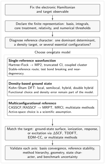
An electronic-structure method is chosen after the Hamiltonian, finite representation, target state, and observable are declared. The branches organize reference character and target type; they are not a universal accuracy ranking. Every route ends in separate representation, method, state-character, and property validation.

Hartree–Fock

One optimized determinant

Hartree–Fock restricts the normalized trial state to one Slater determinant:

$$|\Phi_0\rangle = \frac{1}{\sqrt{N!}} \det[\phi_i(\mathbf x_j)].$$

The orbitals are varied to make

$$E_{\mathrm{HF}} = \min_{\Phi\ \mathrm{determinant}} \langle\Phi|\hat H_{\mathrm e}|\Phi\rangle.$$

For the same Hamiltonian and complete one-particle space,

$$E_{\mathrm{exact}} \leq E_{\mathrm{HF}}.$$

This upper-bound statement applies to the optimized total energy. It does not make every orbital energy, density-derived property, or energy difference an upper bound.

What the reference captures

The determinant enforces fermionic antisymmetry and therefore contains exchange exactly within the chosen orbital space. Its orbitals relax self-consistently in the mean field of the others. Hartree–Fock often supplies:

• a useful closed-shell equilibrium reference;
• occupied and virtual orbital subspaces;
• a zeroth-order state for perturbation, CI, and coupled cluster;
• qualitative charge, symmetry, and bonding information;
• a diagnostic baseline for correlation.

It does not omit electron–electron repulsion. It replaces the fully correlated many-electron response by the best state within the one-determinant manifold.

Restricted, unrestricted, and generalized forms

Restricted closed-shell Hartree–Fock pairs $\alpha$ and $\beta$ electrons in the same spatial orbitals. Unrestricted Hartree–Fock permits different spatial orbitals for the two spin projections. Generalized Hartree–Fock permits still broader spinor mixing.

Relaxing a restriction can lower the variational energy, but the resulting state may no longer be an eigenstate of $\hat S^2$. Broken symmetry can be a useful mean-field diagnostic; it is not automatically a faithful spin-pure wavefunction.

Characteristic failure modes

One determinant is least reliable when:

• bonds are stretched toward competing covalent structures;
• several orbital occupations become nearly degenerate;
• low-spin transition-metal states compete;
• open shells require several spin couplings;
• dispersion or short-range pair correlation controls an energy difference;
• an excited state is not adiabatically connected to the ground-state determinant.

SCF convergence only means that a stationary solution was found. Stability analysis and alternative initial guesses are needed to test whether it is the intended minimum.

Configuration Interaction

Linear expansion in determinants

Configuration interaction expands the state in determinants or symmetry-adapted configuration-state functions:

$$|\Psi_{\mathrm{CI}}\rangle = \sum_I c_I|\Phi_I\rangle.$$

In a fixed finite orbital space, diagonalizing the Hamiltonian over every determinant in the selected symmetry sector gives full CI:

$$\mathbf H\mathbf c = E\mathbf c.$$

FCI is variational and invariant under any unitary change of orbital basis within the same finite one-particle space. Its dimension grows combinatorially. For $K$ spatial orbitals and fixed $N_\alpha,N_\beta$,

$$D = \binom{K}{N_\alpha} \times \binom{K}{N_\beta}.$$

This rapid growth makes FCI a benchmark for small systems and spaces, not a general molecular algorithm.

Excitation-rank truncation

Starting from a reference determinant,

$$|\Psi_{\mathrm{CISD}}\rangle = \left( c_0+\hat C_1+\hat C_2 \right)|\Phi_0\rangle$$

retains single and double substitutions. CISD is variational within its selected space, but the missing disconnected higher excitations make it not size extensive.

For two noninteracting fragments, a double excitation on each fragment is a quadruple excitation relative to the product reference. A fragmentwise CISD product contains that term; supermolecular CISD does not. The error therefore grows improperly with the number of separated fragments.

Two related criteria should be distinguished:

$$E(A\cdots B) \longrightarrow E(A)+E(B)$$

at infinite separation is size consistency, while proportional scaling of the energy with the number of identical noninteracting replicas is size extensivity. Usage is not perfectly uniform across the literature. Ordinary excitation-rank-truncated CI violates the disconnected-product structure behind both criteria.

Where CI remains useful

CI is valuable when:

• a compact determinant space has direct interpretive value;
• several low-lying roots are needed from one Hermitian eigenproblem;
• selected-CI or active-space strategies identify important configurations;
• FCI-quality benchmarks are possible;
• transition moments benefit from straightforward left and right eigenvectors of the same Hermitian matrix.

Coefficients depend on orbital choice and normalization conventions. A small coefficient does not prove that a configuration is physically irrelevant, especially when many individually small terms contribute collectively.

Coupled Cluster

Exponential ansatz

Single-reference coupled cluster writes

$$\begin{aligned} |\Psi_{\mathrm{CC}}\rangle &= e^{\hat T}|\Phi_0\rangle, \\ \hat T &= \hat T_1+\hat T_2+\hat T_3+\cdots. \end{aligned}$$

Even if $\hat T$ is truncated, the exponential generates disconnected products. For example,

$$e^{\hat T_2} = 1+\hat T_2+\frac12\hat T_2^2+\cdots,$$

so simultaneous double excitations on separated fragments appear through $\hat T_2^2$. This factorization is the structural reason truncated coupled-cluster energies can be size extensive under the usual separated-fragment conditions.

Projected nonlinear equations

Define the similarity-transformed Hamiltonian

$$\bar H = e^{-\hat T}\hat H_{\mathrm e}e^{\hat T}.$$

The energy and amplitudes satisfy projected equations such as

$$E_{\mathrm{CC}} = \langle\Phi_0|\bar H|\Phi_0\rangle,$$

and

$$0 = \langle\Phi_\mu|\bar H|\Phi_0\rangle$$

for the included excitation manifold. Because $\bar H$ is generally non-Hermitian, the energy is not a variational upper bound.

Practical hierarchy

Common single-reference levels include:

• CCSD: singles and doubles amplitudes;
• CCSD(T): a perturbative estimate of connected triples added to CCSD;
• CCSDT and beyond: iterative higher excitations at steep cost;
• EOM-CC or linear-response CC: excitation, ionization, attachment, and response sectors built around a coupled-cluster reference.

For dense canonical-orbital textbook implementations, representative formal costs are

$$\begin{aligned} \mathrm{MP2}&:\ O(K^5),\\ \mathrm{CCSD}&:\ O(K^6),\\ \mathrm{CCSD(T)}&:\ O(K^7), \end{aligned}$$

when occupied and virtual dimensions grow together. Memory, prefactors, integral transformations, locality, sparsity, and target properties can dominate real cost. Scaling exponents are not portable timing predictions.

Strengths and cautions

Coupled cluster is often highly accurate for energy differences around a stable single-reference state. Its advantages do not make it black-box exact:

• nonvariational energies can lie below the exact finite-basis energy;
• multiple nonlinear solutions can exist;
• large amplitudes or unstable references signal possible breakdown;
• stretched bonds and near-degeneracies can require high excitation ranks;
• analytic properties require a Lagrangian or response construction, not only the right-hand state;
• basis-set and Hamiltonian errors remain.

Agreement between CCSD and CCSD(T) is useful evidence, not a universal proof of convergence.

Density-Functional Theory

Ground-state density as the basic variable

For a fixed external potential and nondegenerate ground state, the Hohenberg–Kohn framework establishes that the ground-state density determines the external potential up to an additive constant and that the exact energy is obtained by minimizing a density functional:

$$E_0 = \min_{n\to N} \left[ F[n] +\int v_{\mathrm{ext}}(\mathbf r)n(\mathbf r)\,d^3r \right].$$

Kohn–Sham DFT introduces a noninteracting reference system with the same ground-state density. Its energy decomposition is

$$\begin{aligned} E[n] ={}& T_s[n] +\int v_{\mathrm{ext}}(\mathbf r)n(\mathbf r)\,d^3r\\ &+E_{\mathrm H}[n] +E_{\mathrm{xc}}[n] +E_{\mathrm{NN}}. \end{aligned}$$

The orbitals satisfy

$$\begin{aligned} \hat h_{\mathrm{KS}}[n] ={}&-\frac12\nabla^2+v_{\mathrm{ext}}\\ &+v_{\mathrm H}[n]+v_{\mathrm{xc}}[n],\\ \hat h_{\mathrm{KS}}[n]\varphi_i ={}&\varepsilon_i\varphi_i. \end{aligned}$$

with

$$n(\mathbf r) = \sum_{i\in\mathrm{occ}}|\varphi_i(\mathbf r)|^2$$

for a closed-shell-like notation adjusted as needed for spin and occupations.

Exact framework, approximate functional

The exact functional is unknown for general molecular systems. Practical DFT is therefore labeled by the exchange–correlation approximation and other choices:

• local-density approximations;
• generalized-gradient approximations;
• meta-GGAs with additional local ingredients;
• global or range-separated hybrids with nonlocal exchange;
• double hybrids with perturbative correlation;
• dispersion corrections or nonlocal correlation models.

Two calculations called “DFT” can make materially different approximations. Functional names are part of the physical model, not implementation decoration.

What Kohn–Sham orbitals mean

Kohn–Sham orbitals reproduce the density of an auxiliary noninteracting system. They are not generally electron removal or addition states. For the exact functional, the highest occupied eigenvalue has a special ionization relation under appropriate conditions, but the entire orbital spectrum is not a measured excitation spectrum.

The fundamental gap obeys the exact bookkeeping relation

$$\begin{aligned} E_{\mathrm g}^{\mathrm{fund}} &=I-A\\ &= \left( \varepsilon_{\mathrm{LUMO}} -\varepsilon_{\mathrm{HOMO}} \right) +\Delta_{\mathrm{xc}}, \end{aligned}$$

where $\Delta_{\mathrm{xc}}$ is the derivative discontinuity. Approximate functionals can additionally suffer density-driven and functional-driven errors.

Characteristic molecular failures

The severity depends on the functional and target, but recurring risks include:

• self-interaction and delocalization error;
• poor long-range charge transfer without suitable asymptotics;
• fractional-charge and fractional-spin errors;
• missing or double-counted dispersion;
• strong dependence on spin state and symmetry breaking;
• multireference bond dissociation;
• functional-specific barrier, thermochemistry, and response errors;
• grid and integration sensitivity for some functionals.

Benchmark performance is domain dependent. A functional validated for main-group equilibrium thermochemistry is not thereby validated for transition-metal spin gaps, Rydberg excitations, or bond cleavage.

Multireference Methods

When one determinant is not enough

A wavefunction has multireference character when several configurations are essential at zeroth order. Typical causes include:

• homolytic bond breaking;
• avoided crossings and conical-intersection regions;
• open-shell singlets;
• transition-metal valence manifolds;
• diradicals and polyradicals;
• nearly degenerate valence and Rydberg configurations;
• several states that must remain balanced along a geometry path.

This is often called static, strong, or near-degeneracy correlation. Terminology varies, but the operational issue is stable: perturbing around one determinant becomes poorly conditioned because important configurations are too close in energy.

Active-space construction

Complete-active-space self-consistent field partitions orbitals into:

• inactive orbitals, constrained to be doubly occupied;
• active orbitals, whose occupations are distributed in a complete CI expansion;
• external orbitals, unoccupied in the reference expansion.

The state is

$$|\Psi_{\mathrm{CASSCF}}\rangle = \sum_{I\in\mathrm{CAS}}c_I|\Phi_I\rangle,$$

while both $c_I$ and orbital rotations are optimized. A notation such as CAS$(n_{\mathrm e},n_{\mathrm o})$ declares the number of active electrons and active spatial orbitals.

CASSCF captures the principal configurational rearrangements inside the chosen active space. It does not recover all dynamic correlation outside that space.

Choosing an active space

The active orbitals should follow the physical process:

• include bonding and antibonding partners for a breaking bond;
• include nearly degenerate open-shell orbitals;
• include the orbitals needed to describe all targeted states consistently;
• preserve chemically and symmetry-related partners;
• inspect occupations, entropies, and orbital character across the entire geometry path.

An active space chosen from one equilibrium geometry can become unbalanced elsewhere. State-averaged optimization can maintain a common orbital description for several roots, but the weights are additional modeling choices.

Recovering dynamic correlation

Common extensions include:

• multireference perturbation theories such as CASPT2 or NEVPT2;
• multireference configuration interaction;
• internally contracted variants;
• selected-CI, DMRG, or other active-space solvers for larger spaces;
• multistate effective-Hamiltonian treatments near interacting roots.

These methods differ in size consistency, intruder-state behavior, contraction, invariance, zeroth-order Hamiltonian, and state-coupling conventions. “CASSCF plus second order” is not a complete reproducibility statement.

Diagnostics are evidence, not verdicts

Natural-orbital occupations far from $0$ or $2$, large coupled-cluster amplitudes, small orbital gaps, unstable Hartree–Fock solutions, and strong method dependence can all signal multireference character. No universal scalar threshold classifies every molecule and property. The decisive test is whether a balanced state model converges the target observable across relevant geometries and states.

Excited States

Specify the energy being compared

At a ground-state geometry $\mathbf R_0$, a vertical excitation energy is

$$\Delta E_{\mathrm{vert}} = E_k(\mathbf R_0)-E_0(\mathbf R_0).$$

An adiabatic excitation energy compares relaxed minima:

$$\Delta E_{\mathrm{ad}} = E_k(\mathbf R_k)-E_0(\mathbf R_0).$$

An experimental band maximum, $0$–$0$ energy, onset, or photoelectron peak can differ from both because of zero-point motion, vibronic structure, temperature, lifetime, and environment.

Method families for excited states

Different constructions answer different excited-state questions:

• CIS supplies a simple single-excitation model but lacks ground-state correlation and doubles-dominated states.
• TDDFT linear response is often efficient for many valence excitations, with accuracy controlled by the functional, kernel, state character, and reference; standard adiabatic kernels do not describe genuine double-excitation character reliably.
• EOM-CC and linear-response CC provide systematic single-reference excited, ionized, or electron-attached sectors.
• $\Delta$SCF optimizes an excited occupancy directly but requires careful state tracking and symmetry control.
• state-averaged CASSCF and multistate correlation methods treat several interacting configurations and surfaces on a common footing.

No method is selected by excitation energy alone. Valence, Rydberg, charge-transfer, double-excitation, core-excited, spin-flip, and ionized states place different demands on basis functions and ansätze.

Intensities and state character

An excitation energy does not determine whether a transition is visible. In the electric-dipole approximation, an oscillator strength is proportional to an energy gap times a transition moment:

$$f_{0k} \propto \Delta E_{0k} \sum_{\alpha=x,y,z} \left| \langle\Psi_k|\hat\mu_\alpha|\Psi_0\rangle \right|^2.$$

State symmetry, spin, polarization, vibronic coupling, and the quality of left and right response states matter. Comparing only energies can miss a qualitatively wrong assignment.

Oscillator Strengths gives the normalized electronic and vibronic definitions, polarization and degeneracy averages, sum rules, and absorption-area conventions.

Intersections and changing character

Near an avoided crossing or conical intersection, several states must be represented with balanced accuracy. A state-specific method can become discontinuous or swap character. Smooth energies alone do not guarantee smooth wavefunctions, derivative couplings, or observables. Nonadiabatic Coupling develops that coupled-surface dynamics problem. Conical Intersections owns exact-degeneracy geometry, branching-plane tests, seam optimization, and MECI interpretation.

Accuracy, Cost, and Interpretation

Typical dense-algebra costs

Formal scaling is useful for orientation when its variables and implementation class are stated. With a generic orbital dimension $K$:

• Hartree–Fock and hybrid-exchange formation are often associated with quartic integral structure, though modern algorithms vary widely;
• semilocal Kohn–Sham DFT adds numerical quadrature and is often lower cost than correlated wavefunction methods;
• MP2 is conventionally $O(K^5)$;
• CISD and CCSD are conventionally $O(K^6)$;
• perturbative triples in CCSD(T) are conventionally $O(K^7)$;
• FCI and complete active-space dimensions grow combinatorially.

These labels omit prefactors, memory, disk traffic, derivative order, number of states, basis diffuseness, symmetry, locality, parallel efficiency, and integral approximations. A nominally lower-scaling method can be slower for the system and property at hand.

Method profiles

Hartree–Fock

• State model: one optimized determinant.
• Strong use: reference orbitals, qualitative exchange, stable closed-shell baselines.
• Main warning: missing dynamic correlation and failing near degeneracy.

Truncated CI

• State model: linear selected excitation space.
• Strong use: interpretable roots and finite-space variational energies.
• Main warning: ordinary excitation-rank truncations are not size extensive.

Single-reference coupled cluster

• State model: exponential excitations from one determinant.
• Strong use: high-accuracy equilibrium energetics when the reference is stable.
• Main warning: nonvariational and vulnerable to strong multireference character.

Kohn–Sham DFT

• State model: approximate density functional represented by auxiliary orbitals.
• Strong use: broad molecular sizes, structures, densities, and screening.
• Main warning: functional- and domain-dependent errors; orbital eigenvalues require care.

CASSCF and multireference extensions

• State model: optimized orbitals plus several essential configurations.
• Strong use: bond breaking, interacting states, open-shell manifolds.
• Main warning: active-space dependence and incomplete dynamic correlation.

Convergence is multidimensional

A credible result varies one approximation axis at a time.

1. Numerical convergence: SCF residuals, integral thresholds, grids, geometry gradients.
2. Representation convergence: basis cardinality, augmentation, core treatment.
3. Correlation convergence: excitation rank, active space, perturbative correction.
4. State convergence: root tracking, symmetry, spin purity, state averaging.
5. Hamiltonian convergence: scalar relativity, spin–orbit coupling, finite mass, environment.
6. Observable convergence: analytic response versus finite difference, origin and gauge checks where relevant.

A single large calculation does not replace a convergence sequence.

Energy differences need balanced errors

For a reaction

$$\sum_r\nu_r R_r \longrightarrow \sum_p\nu_p P_p,$$

the electronic reaction energy is

$$\Delta E_{\mathrm{rxn}} = \sum_p\nu_p E_p -\sum_r\nu_r E_r.$$

Accuracy depends on correlated cancellation among all species. Use the same Hamiltonian, compatible basis strategy, state definitions, and convergence thresholds. Isodesmic or homodesmotic reactions can improve cancellation, but they change the thermochemical cycle rather than making the underlying electronic energies exact.

Interpret invariant quantities first

Total energies, densities, expectation values, transition amplitudes, and properly defined reduced density matrices are state-level objects. Canonical orbitals and individual CI coefficients can change under allowed orbital rotations. Localized orbitals, charges, bond orders, and energy decompositions depend on additional definitions.

Interpretation is strongest when:

• the quantity is invariant under irrelevant basis rotations;
• its operator or partition is stated;
• multiple complementary diagnostics agree;
• the conclusion survives reasonable method and representation changes.

Reproducibility checklist

A molecular electronic-structure result should report:

• molecular geometry or geometry source;
• charge, multiplicity, symmetry constraints, and state label;
• electronic Hamiltonian, relativity, effective core potentials, and frozen-core choices;
• orbital and auxiliary bases, including diffuse or core–valence augmentation;
• method, reference type, functional, active space, and state-averaging weights;
• convergence thresholds, integration grid, and stability checks;
• property definition and whether it is vertical, adiabatic, relaxed, or response-based;
• software and version when numerical details matter;
• basis, method, and state-character convergence evidence;
• comparison data with uncertainty and matched physical conditions.

The NIST Computational Chemistry Comparison and Benchmark Database is one useful source of paired gas-phase experimental and calculated data. Its coverage and property definitions still have to match the question being asked.

Worked Example: H₂ Dissociation

The minimal-basis hydrogen molecule exposes the boundary between dynamic and static correlation.

Bonding reference near equilibrium

Ignoring overlap for the limiting argument, define normalized atomic orbitals $A$ and $B$ and molecular orbitals

$$\sigma_g = \frac{A+B}{\sqrt2}, \qquad \sigma_u = \frac{A-B}{\sqrt2}.$$

The spatial products below are understood to multiply the normalized singlet spin function.

Near equilibrium, the closed-shell configuration

$$|\sigma_g^2\rangle$$

is dominant. Correlation methods built around that determinant can efficiently improve the energy.

Ionic contamination at large separation

Its spatial product is

$$\begin{aligned} \sigma_g(1)\sigma_g(2) = \frac12\big[&\\ &A(1)A(2)\\ &+A(1)B(2)\\ &+B(1)A(2)\\ &+B(1)B(2)\big]. \end{aligned}$$

The middle terms are covalent: one electron lies on each atom. The first and last are ionic. At dissociation, a spin-singlet neutral molecule should approach the covalent Heitler–London combination, but restricted Hartree–Fock retains equal ionic weight.

A second configuration repairs the limit

The antibonding pair has

$$\begin{aligned} \sigma_u(1)\sigma_u(2) = \frac12\big[&\\ &A(1)A(2)\\ &-A(1)B(2)\\ &-B(1)A(2)\\ &+B(1)B(2)\big]. \end{aligned}$$

Therefore

$$\begin{gathered} \frac{1}{\sqrt2} \left( |\sigma_g^2\rangle -|\sigma_u^2\rangle \right)\\ \longrightarrow\\ \frac{1}{\sqrt2} \left[ A(1)B(2)+B(1)A(2) \right] \end{gathered}$$

as the overlap vanishes. The ionic terms cancel. Both configurations become equally important, so the problem is multireference even in this tiny basis.

What different methods do

• Restricted Hartree–Fock preserves spin and spatial symmetry but dissociates incorrectly.
• Unrestricted Hartree–Fock can lower the energy by localizing opposite spins, but the determinant breaks spin symmetry.
• Finite-order single-reference perturbation and coupled-cluster methods become stressed as the orbital gap closes.
• Minimal-space FCI or CASSCF$(2,2)$ contains both configurations and gives the correct qualitative singlet dissociation.
• Dynamic correlation and basis completeness remain separate corrections after the two-configuration structure is repaired.

Hydrogen Molecule owns the broader molecular derivation and bonding physics. Here the example diagnoses method choice.

A Practical Method-Selection Workflow

1. Declare the target

State the geometry range, charge, spin, symmetry, state, observable, and desired uncertainty. “Find the electronic structure” is not a sufficiently bounded task.

2. Choose the Hamiltonian

Decide whether the nonrelativistic Born–Oppenheimer electronic Hamiltonian is adequate. Add scalar relativity, spin–orbit coupling, external fields, embedding, or environmental terms only with a declared convention.

3. Design the representation

Choose basis functions for the property: polarization for bonding response, diffuse functions for tails, core–valence flexibility for core correlation, and compatible relativistic or effective-core models where needed.

4. Diagnose reference character

Inspect orbital occupations and gaps, alternative SCF solutions, spin contamination, coupled-cluster amplitudes where available, and behavior along the full geometry path. Do not diagnose only at the easiest geometry.

5. Match the method to the state

• Stable single-reference ground state: test HF-based correlation or an appropriately benchmarked functional.
• Large-system density or structure screening: test a functional family suited to the domain.
• Bond breaking or competing configurations: use a balanced multireference model.
• Excited state: match the method to valence, Rydberg, charge-transfer, double-excitation, ionized, or core character.

6. Converge independent axes

Run at least one meaningful basis sequence and one meaningful method or active-space sequence. Tighten numerical thresholds beyond the target uncertainty.

7. Validate without tuning to one answer

Compare several observables or benchmark classes, not only the number used to choose the method. Preserve a distinction between calibration data and a genuine prediction test.

Common Mistakes

“A bigger basis is a better method”

A basis enlarges the representation. It does not change a one-determinant ansatz into a correlated or multireference state.

“Full CI is exact”

FCI is exact only within the stated finite orbital space and Hamiltonian.

“Hartree–Fock neglects electron repulsion”

Hartree–Fock includes direct and exchange effects self-consistently. It misses correlation outside the determinant manifold.

“CCSD(T) is always the gold standard”

It is exceptionally effective for many stable single-reference molecules near equilibrium. Strong near-degeneracy, difficult excited states, heavy-element Hamiltonians, and property-specific demands can invalidate the slogan.

“DFT is one method”

Practical predictions depend on the exchange–correlation approximation, density, basis, grid, dispersion model, spin treatment, and property formalism.

“Kohn–Sham orbital gaps are excitation energies”

The auxiliary eigenvalue gap omits the derivative discontinuity in the exact ground-state relation and does not generally equal a neutral optical excitation.

“CASSCF includes all correlation”

CASSCF treats complete configuration interaction only inside the chosen active space while optimizing orbitals. Most external dynamic correlation remains.

“A converged root is the intended state”

SCF and excited-state solvers can converge to unintended stationary points or swap root character.

“Agreement with experiment validates the electronic method”

Cancellation among electronic, basis, geometry, nuclear-motion, relativistic, environmental, and experimental effects can produce agreement for the wrong reason.

“Formal scaling determines actual feasibility”

Memory, prefactors, sparsity, number of states, derivative order, hardware, and implementation alter the crossover.

Exercises

Exercise 1: Count a finite CI sector

A calculation uses $K=7$ spatial orbitals with $N_\alpha=N_\beta=5$. How many Slater determinants lie in this fixed-$M_S$ sector before point-group or spin adaptation?

Solution

Choose the occupied spatial orbitals independently for the $\alpha$ and $\beta$ strings:

$$D = \binom{7}{5}\binom{7}{5} = 21^2 = 441.$$

This is not the number of spin-adapted configuration-state functions, and it is smaller than an unrestricted count over all $M_S$ sectors. The example shows how symmetry-sector declarations affect the many-electron dimension.

Exercise 2: Remove the overlap metric

Suppose $\mathbf S$ is positive definite and

$$\mathbf F\mathbf C = \mathbf S\mathbf C\boldsymbol\varepsilon.$$

Show how symmetric orthogonalization turns this into an ordinary Hermitian eigenproblem.

Solution

Diagonalize the overlap:

$$\mathbf S = \mathbf U\mathbf s\mathbf U^\dagger,$$

and define

$$\mathbf X = \mathbf S^{-1/2} = \mathbf U\mathbf s^{-1/2}\mathbf U^\dagger.$$

Write $\mathbf C=\mathbf X\widetilde{\mathbf C}$ and left-multiply by $\mathbf X^\dagger$. Since

$$\mathbf X^\dagger\mathbf S\mathbf X = \mathbf I,$$

one obtains

$$\widetilde{\mathbf F}\widetilde{\mathbf C} = \widetilde{\mathbf C}\boldsymbol\varepsilon, \qquad \widetilde{\mathbf F} = \mathbf X^\dagger\mathbf F\mathbf X.$$

Small eigenvalues of $\mathbf S$ make $\mathbf S^{-1/2}$ large, explaining the numerical danger of near-linear dependence.

Exercise 3: Separate variational and basis statements

Two FCI calculations use nested one-particle spaces $\mathcal B_1\subset\mathcal B_2$ for the same Hamiltonian and symmetry sector. What can be concluded about their ground-state energies? What cannot be concluded about a dipole moment?

Solution

Every determinant available in $\mathcal B_1$ is also available in $\mathcal B_2$, so the Rayleigh–Ritz variational spaces are nested:

$$E_{\mathrm{FCI}}(\mathcal B_2) \leq E_{\mathrm{FCI}}(\mathcal B_1).$$

Both remain upper bounds to the exact ground-state energy of the declared Hamiltonian.

A dipole expectation value has no analogous one-sided variational bound. It may approach its complete-basis value nonmonotonically even while the energy decreases monotonically.

Exercise 4: Repair the H₂ dissociation limit

Using

$$\sigma_g=\frac{A+B}{\sqrt2}, \qquad \sigma_u=\frac{A-B}{\sqrt2},$$

show which linear combination of $|\sigma_g^2\rangle$ and $|\sigma_u^2\rangle$ removes the ionic $A(1)A(2)$ and $B(1)B(2)$ terms.

Solution

Expanding the two products gives equal ionic terms and opposite covalent terms. Their difference is

$$\begin{aligned} &\sigma_g(1)\sigma_g(2) -\sigma_u(1)\sigma_u(2)\\ &\qquad= A(1)B(2)+B(1)A(2). \end{aligned}$$

After normalization at vanishing overlap,

$$|\Psi_{\mathrm{cov}}\rangle = \frac{1}{\sqrt2} \left( |\sigma_g^2\rangle -|\sigma_u^2\rangle \right).$$

The need for two equally weighted configurations is the minimal signature of static correlation in the stretched singlet.

Exercise 5: Why CISD is not size extensive

Fragments $A$ and $B$ do not interact. Each has an important double-excitation operator, $\hat C_2^A$ or $\hat C_2^B$. Explain why the product of fragment CISD states contains a term absent from supermolecular CISD, and why an exponential doubles ansatz can contain it.

Solution

The fragment product contains

$$\left(1+\hat C_2^A\right) \left(1+\hat C_2^B\right) |\Phi_A\Phi_B\rangle.$$

Expanding gives

$$\left( 1+\hat C_2^A+\hat C_2^B +\hat C_2^A\hat C_2^B \right) |\Phi_A\Phi_B\rangle.$$

The final term is a quadruple excitation relative to the product reference, so a supermolecular CISD truncation omits it.

For coupled cluster,

$$e^{\hat T_2^A+\hat T_2^B} = e^{\hat T_2^A}e^{\hat T_2^B}$$

because operators on separated fragments commute. The exponential therefore generates the disconnected product through its quadratic and higher terms.

Exercise 6: Evaluate a counterpoise correction

For a dimer, suppose

$$\begin{aligned} E_{AB}^{AB}&=-200.120\,E_{\mathrm h},\\ E_A^{AB}&=-100.052\,E_{\mathrm h},\\ E_B^{AB}&=-100.051\,E_{\mathrm h}, \end{aligned}$$

while $E_A^A=E_B^B=-100.050\,E_{\mathrm h}$. Compute the raw and counterpoise interaction energies.

Solution

The raw value is

$$\begin{aligned} \Delta E_{\mathrm{int}}^{\mathrm{raw}} ={}&-200.120\\ &-(-100.050)-(-100.050)\\ ={}& -0.020\,E_{\mathrm h}. \end{aligned}$$

The counterpoise value is

$$\begin{aligned} \Delta E_{\mathrm{int}}^{\mathrm{CP}} ={}&-200.120\\ &-(-100.052)-(-100.051)\\ ={}& -0.017\,E_{\mathrm h}. \end{aligned}$$

Basis borrowing overbinds by $0.003\,E_{\mathrm h}$ in this example. The counterpoise result can still contain correlation, basis-incompleteness, geometry, and Hamiltonian errors.

Exercise 7: Choose state models

Choose a first method family and one decisive validation check for each task:

1. an equilibrium closed-shell reaction energy with no near-degeneracy evidence;
2. symmetric homolytic bond cleavage;
3. a long-range charge-transfer excitation;
4. two nearly intersecting excited surfaces.

Solution

1. A single-reference hierarchy such as coupled cluster, or a carefully benchmarked functional for larger systems, is reasonable. Check basis and correlation convergence and test reference stability.
2. Use an active-space or other multireference description containing bonding and antibonding orbitals. Check natural occupations and correct separated-fragment limits across the full coordinate.
3. Use a method with appropriate long-range response, such as a validated range-separated TDDFT approximation or EOM-CC when feasible. Check donor–acceptor separation behavior and diffuse-basis convergence.
4. Use a balanced multistate multireference treatment. Check state character, energy-gap topology, and invariance to reasonable state-averaging and active-space changes.

The answers are families, not software recipes. System size, Hamiltonian, and target uncertainty can change the practical choice.

Exercise 8: Fundamental and Kohn–Sham gaps

For a molecule, $I=8.8\,\mathrm{eV}$, $A=0.5\,\mathrm{eV}$, and an exact Kohn–Sham calculation would have

$$\varepsilon_{\mathrm{LUMO}} -\varepsilon_{\mathrm{HOMO}} = 6.9\,\mathrm{eV}.$$

Find the fundamental gap and derivative discontinuity.

Solution

The fundamental gap is

$$E_{\mathrm g}^{\mathrm{fund}} = I-A = 8.3\,\mathrm{eV}.$$

Using

$$E_{\mathrm g}^{\mathrm{fund}} = E_{\mathrm g}^{\mathrm{KS}} +\Delta_{\mathrm{xc}},$$

gives

$$\Delta_{\mathrm{xc}} = 8.3-6.9 = 1.4\,\mathrm{eV}.$$

This exact bookkeeping relation does not imply that a practical approximate functional supplies either term exactly.

Key Takeaways

• An electronic-structure result is defined by Hamiltonian, representation, state model, property model, and numerical realization.
• Basis incompleteness, correlation truncation, multireference character, and missing physical terms are different error axes.
• Hartree–Fock is the best one-determinant state, not a no-interaction model.
• FCI is exact only in a stated finite space; truncated CI is variational but generally not size extensive.
• Coupled cluster gains size-extensive factorization from its exponential ansatz but is nonvariational and reference dependent.
• Kohn–Sham DFT is an exact ground-state framework used with approximate functionals whose domain and density errors must be tested.
• CASSCF balances essential configurations in a chosen active space but leaves much dynamic correlation outside it.
• Excited-state method choice depends on state character, not only the expected excitation energy.
• Trust comes from independent convergence checks, matched benchmarks, and complete provenance rather than a prestigious acronym.

Cross-Links

• Electronic Structure Methods Map turns the formal method families into an operational choice, diagnostics, cost, convergence, and validation workflow.
• Molecular Quantum Mechanics places electronic states in the electronic–vibrational–rotational hierarchy.
• Molecular Hamiltonian derives the all-particle Coulomb operator and center-of-mass separation.
• Born–Oppenheimer in Molecules explains how fixed-geometry electronic eigenvalues become nuclear potential surfaces.
• Potential Energy Surfaces owns minima, saddle points, reaction paths, crossings, and surface validation.
• Nonadiabatic Coupling connects balanced multistate electronic structure to derivative couplings, vibronic models, and molecular dynamics.
• Conical Intersections develops seam geometry, branching-plane diagnostics, MECI optimization, and method-specific failure modes.
• Molecular Orbitals owns LCAO construction, orbital labels, occupations, gaps, and interpretation.
• Valence Bond Theory develops localized spin-coupled structures and their relation to MO expansions.
• Hydrogen Molecule develops the two-electron bond and dissociation problem in detail.
• Chemical Bonding compares energetic, density, force, orbital, and spectroscopic bond diagnostics.
• Molecular Symmetry develops point-group sectors, symmetry-adapted orbitals, and state-label diagnostics.
• Exchange and Correlation separates direct interaction, exchange, and correlation concepts.
• Atomic Correlation Methods Overview applies CI, MBPT, coupled cluster, DFT, and QMC to atomic structure.
• Hartree–Fock Approximation owns the general determinant variational derivation.
• Variational Many-Body States compares ansatz families across interacting quantum systems.
• Entanglement in Quantum Chemistry distinguishes correlation energy, orbital entanglement, and basis-dependent mode partitions.
• Oscillator Strengths converts transition moments into electronic and vibronic spectroscopic strengths.
• Electronic Spectroscopy connects calculated states, surfaces, and transition moments to 0–0 origins, vibronic envelopes, and measured absorption bands.
• Quantum Chemistry Roadmap gives the prerequisite and reading sequence.
• Quantum Chemistry References provides a broader annotated bibliography.
• VQE develops the variational quantum workflow for an already specified finite electronic Hamiltonian and keeps algorithmic error distinct from chemistry-model error.
• Simulation of Quantum Chemistry follows a declared molecular model through active-space construction, fermion-to-qubit encoding, state preparation, solver choice, resource accounting, and chemical validation.
• Quantum Chemistry Case Studies compares executed molecular calculations, active-space approximations, phase-estimation demonstrations, and fault-tolerant resource scenarios.

References

• T. Helgaker, P. Jørgensen, and J. Olsen, Molecular Electronic-Structure Theory, Wiley, 2000 — comprehensive wavefunction theory, basis sets, response, and molecular properties.
• A. Szabo and N. S. Ostlund, Modern Quantum Chemistry: Introduction to Advanced Electronic Structure Theory, Dover, 1996 — standard derivations of Hartree–Fock and post-Hartree–Fock methods.
• I. Shavitt and R. J. Bartlett, Many-Body Methods in Chemistry and Physics, Cambridge University Press, 2009 — MBPT and coupled-cluster formalism.
• F. Jensen, Introduction to Computational Chemistry, 3rd ed., Wiley, 2017 — practical basis, method, property, and validation perspective.
• C. J. Cramer, Essentials of Computational Chemistry, 2nd ed., Wiley, 2004 — model chemistry, thermochemistry, solvation, and interpretation.
• C. C. J. Roothaan, “New Developments in Molecular Orbital Theory,” Reviews of Modern Physics 23, 69–89 (1951) — finite-basis self-consistent-field formulation.
• T. H. Dunning Jr., “Gaussian Basis Sets for Use in Correlated Molecular Calculations. I,” Journal of Chemical Physics 90, 1007–1023 (1989) — correlation-consistent basis construction.
• S. F. Boys and F. Bernardi, “The Calculation of Small Molecular Interactions by the Differences of Separate Total Energies. Some Procedures with Reduced Errors,” Molecular Physics 19, 553–566 (1970) — counterpoise treatment of basis-set superposition.
• R. J. Bartlett and M. Musiał, “Coupled-Cluster Theory in Quantum Chemistry,” Reviews of Modern Physics 79, 291–352 (2007) — authoritative coupled-cluster review.
• P. Hohenberg and W. Kohn, “Inhomogeneous Electron Gas,” Physical Review 136, B864–B871 (1964) — ground-state density-functional foundations.
• W. Kohn and L. J. Sham, “Self-Consistent Equations Including Exchange and Correlation Effects,” Physical Review 140, A1133–A1138 (1965) — Kohn–Sham construction.
• E. Runge and E. K. U. Gross, “Density-Functional Theory for Time-Dependent Systems,” Physical Review Letters 52, 997–1000 (1984) — time-dependent density-functional foundation.
• B. O. Roos, P. R. Taylor, and P. E. M. Siegbahn, “A Complete Active Space SCF Method Using a Density Matrix Formulated Super-CI Approach,” Chemical Physics 48, 157–173 (1980) — original CASSCF formulation.
• J. F. Stanton and R. J. Bartlett, “The Equation of Motion Coupled-Cluster Method. A Systematic Biorthogonal Approach to Molecular Excitation Energies, Transition Probabilities, and Excited State Properties,” Journal of Chemical Physics 98, 7029–7039 (1993) — EOM-CC for excitation energies and properties.
• M. Schreiber, M. R. Silva-Junior, S. P. A. Sauer, and W. Thiel, “Benchmarks for Electronically Excited States: CASPT2, CC2, CCSD, and CC3,” Journal of Chemical Physics 128, 134110 (2008) — comparative excited-state benchmarks.
• R. D. Johnson III, editor, NIST Computational Chemistry Comparison and Benchmark Database, Standard Reference Database 101, release 22 (2022), DOI 10.18434/T47C7Z — gas-phase experimental and computed benchmark data with property-specific comparisons.