Electronic Spectroscopy

Electronic spectroscopy observes transitions between electronic energy levels of atoms, ions, molecules, or condensed-phase species. An isolated atom often produces a set of narrow electronic lines split by angular momentum, spin–orbit, hyperfine, Zeeman, or Stark structure. A molecule usually produces vibronic bands because each electronic state supports vibration and rotation, and because its equilibrium geometry and force constants can change upon electronic excitation.

The central inference chain is

$$\begin{gathered} \begin{matrix} \text{electronic states} \\ \text{and nuclear potentials} \end{matrix} \\ \downarrow \\ \begin{matrix} \text{transition moments} \\ \text{and vibronic overlaps} \end{matrix} \\ \downarrow \\ \text{line or band strengths} \\ \downarrow \\ \begin{matrix} \text{broadening, propagation,} \\ \text{and detection} \end{matrix} \\ \downarrow \\ \text{recorded electronic spectrum}. \end{gathered}$$

Each arrow carries assumptions. A peak coordinate need not equal an electronic-state minimum gap. A symmetry-allowed transition need not be intense. A broad band need not be a single transition. An excitation spectrum need not reproduce an absorption spectrum. Electronic spectroscopy becomes quantitatively trustworthy when these layers are kept separate.

Canonical Scope

This page owns the spectrum-facing treatment of:

• electronic transition energies in atoms and molecules;
• the distinction among adiabatic, 0–0, vertical, and band-maximum energies;
• Franck–Condon factors and displaced-oscillator progressions;
• vibronic, rotational, hot-band, and continuum structure;
• Condon and Herzberg–Teller intensity mechanisms;
• electronic spin, parity, and molecular-symmetry rules;
• absorption-band interpretation; and
• the limited conditions connecting absorption, excitation, and fluorescence spectra.

Nearby pages retain complementary canonical roles:

• Electronic Structure Overview owns the choice and validation of electronic-structure methods.
• Potential Energy Surfaces owns surface topology, stationary points, reaction paths, and surface representations.
• Born–Oppenheimer in Molecules owns the electronic–nuclear hierarchy and the general molecular transition amplitude.
• Nonadiabatic Coupling owns population transfer among electronic surfaces, vibronic Hamiltonians, wavepacket branching, and photochemical dynamics.
• Oscillator Strengths owns oscillator-strength conventions, sum rules, and conversion between transition moments and integrated strengths.
• Selection Rules in Spectroscopy owns the process-first hierarchy of exact, approximate, and propensity rules.
• Absorption and Emission owns radiative transfer, stimulated versus spontaneous processes, and measurement conventions.
• Line Shapes and Broadening owns homogeneous, inhomogeneous, instrumental, and composite profiles.

The goal here is to assemble those ingredients into a reliable reading of an electronic spectrum.

What Counts as an Electronic Transition?

An electronic transition changes the electronic state of the system. For stationary initial and final states,

$$\widehat H|i\rangle=E_i|i\rangle, \qquad \widehat H|f\rangle=E_f|f\rangle,$$

and one-photon absorption satisfies

$$h\nu = \hbar\omega = E_f-E_i.$$

This equation is exact for the complete system plus a photon in an idealized energy-conserving transition. Its interpretation depends on what the labels $i$ and $f$ contain.

Atomic lines

For an atom or ion, an electronic level label may include configuration, term, total electronic angular momentum, parity, hyperfine angular momentum, and external-field quantum numbers:

$$|\gamma L S J I F M_F;\pi\rangle.$$

Here $\gamma$ denotes remaining configuration and coupling labels. Fine structure separates different $J$ values; hyperfine interactions separate $F$ values; fields can separate magnetic sublevels. The spectrum therefore contains transitions between levels, not merely differences between one-electron orbital energies.

Term Symbol Reference decodes atomic and molecular label conventions, while Atomic Term Symbols, Fine Structure, and Hyperfine Structure develop these labels. The NIST Atomic Spectra Database is an authoritative source for critically evaluated atomic levels, lines, transition probabilities, and related data.

Molecular bands

Within a Born–Oppenheimer description, a molecular state contains electronic, vibrational, rotational, and often spin or parity labels. A useful schematic energy decomposition is

$$\begin{aligned} E_{s v J \alpha} &= T_s + G_s(v) + F_{s v}(J,\alpha) \\ &\quad+ \delta E_{s v J\alpha}, \end{aligned}$$

where:

• $s$ labels an electronic state;
• $T_s$ is a chosen electronic reference energy;
• $G_s(v)$ is a vibrational term value;
• $F_{s v}(J,\alpha)$ contains rotational and projection-dependent structure;
• $\delta E$ collects spin–orbit, spin–rotation, hyperfine, tunneling, nonadiabatic, field, or other corrections required by the resolution.

A molecular electronic transition generally changes both the electronic and vibrational quantum numbers. IUPAC calls such a process a vibronic transition. Rotational quantum numbers usually change as well, so a resolved gas-phase electronic band is more precisely rovibronic.

Energy-scale hierarchy

Typical scales often obey

$$\Delta E_{\mathrm{rot}} \ll \Delta E_{\mathrm{vib}} \ll \Delta E_{\mathrm{el}},$$

but this is an orientation rule, not a theorem. Low-lying electronic states, soft vibrations, heavy-atom spin–orbit splittings, Rydberg series, near degeneracies, and condensed-phase interactions can violate a simple hierarchy. The observed resolution also decides whether the spectrum appears as individual lines, rotational contours, vibronic bands, or a smooth envelope.

The Electronic-Energy Ledger

Several energies are routinely called an “electronic transition energy.” They answer different questions and should not be interchanged.

Let $V_g(Q)$ and $V_e(Q)$ be ground- and excited-state potential-energy surfaces along a nuclear coordinate $Q$, with equilibrium geometries $Q_e''$ and $Q_e'$. Define the minimum-to-minimum electronic gap

$$T_e = V_e(Q_e') - V_g(Q_e'').$$

This is an adiabatic electronic gap between clamped-nuclei minima. It does not yet include vibrational zero-point energies.

The 0–0 transition connects the lowest vibrational levels of the two electronic states:

$$\begin{aligned} E_{00} &= \bigl[ V_e(Q_e')+G_e(0) \bigr] \\ &\quad- \bigl[ V_g(Q_e'')+G_g(0) \bigr]. \end{aligned}$$

Thus

$$\begin{aligned} E_{00} &= T_e+\Delta E_{\mathrm{ZPE}}, \\ \Delta E_{\mathrm{ZPE}} &= G_e(0)-G_g(0). \end{aligned}$$

IUPAC defines zero–zero absorption or emission as a transition between the lowest vibrational levels of two electronic states.

At the ground-state equilibrium geometry, the vertical clamped-nuclei gap is

$$\Delta E_{\mathrm{vert}}^{(g)} = V_e(Q_e'') - V_g(Q_e'').$$

The excited-state reorganization energy

$$\lambda_e = V_e(Q_e'') - V_e(Q_e')$$

gives

$$\Delta E_{\mathrm{vert}}^{(g)} = T_e+\lambda_e.$$

This identity concerns potential energies at stated geometries. A vertical photon absorption begins in a nuclear wavefunction with finite coordinate and momentum spread, not at one classical point.

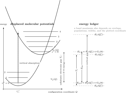
The vertical arrow samples the excited potential near the nuclear configurations occupied before absorption. The adiabatic electronic gap $T_e$, the 0–0 energy $E_{00}$, and a vertical gap are different quantities. A band maximum is not another fundamental gap: it also depends on Franck–Condon factors, populations, line widths, and the spectral coordinate.

Four quantities that are often confused

Quantity	Definition	What it describes
$T_e$	Difference between electronic potential minima	Clamped-nuclei adiabatic electronic gap
$E_{00}$	Difference between lowest vibronic levels	Spectroscopic band origin when observable
$\Delta E_{\mathrm{vert}}$	Electronic energy difference at a specified geometry	Sudden clamped-geometry excitation estimate
Band maximum	Maximum of a measured or modeled spectral density	Overlap, population, width, coordinate, and instrument dependent

The onset of a band is also not automatically $E_{00}$. Weak origin intensity, hot bands, finite signal-to-noise, unresolved rotational structure, inhomogeneous tails, predissociation, or an instrumental threshold can move an operational onset.

A numerical ledger

Suppose $T_e=3.20\ \mathrm{eV}$ and the ground- and excited-state harmonic frequencies are $1400$ and $1000\ \mathrm{cm}^{-1}$. Retaining one effective mode,

$$\Delta E_{\mathrm{ZPE}} = \frac{hc_0}{2} \left( 1000-1400 \right) \mathrm{cm}^{-1}.$$

Using $1\ \mathrm{eV}=8065.54\ \mathrm{cm}^{-1}$ gives

$$\begin{aligned} \Delta E_{\mathrm{ZPE}} &\simeq -0.0248\ \mathrm{eV}, \\ E_{00} &\simeq 3.175\ \mathrm{eV}. \end{aligned}$$

If the excited-state reorganization energy at $Q_e''$ is $0.25\ \mathrm{eV}$, the corresponding clamped-nuclei vertical gap is

$$\Delta E_{\mathrm{vert}}^{(g)} = 3.45\ \mathrm{eV}.$$

Reporting “the excitation energy is $3.45\ \mathrm{eV}$” without the word vertical would erase almost $0.28\ \mathrm{eV}$ of physical bookkeeping.

Franck–Condon Structure

The Franck–Condon principle states, in its quantum formulation, that vibronic intensity is governed by overlap between vibrational wavefunctions when the electronic transition moment is treated as coordinate independent. Its classical “vertical transition” picture is useful, but the overlap integral is the quantitative statement.

The vibronic transition moment

Write Born–Oppenheimer vibronic states schematically as

$$\Psi_{g v''}(r,Q) = \phi_g(r;Q)\chi_{g v''}(Q),$$

and

$$\Psi_{e v'}(r,Q) = \phi_e(r;Q)\chi_{e v'}(Q).$$

For electric-dipole absorption, the vibronic transition moment is

$$\mathbf M_{v'v''} = \int dQ\, \chi_{e v'}^*(Q) \boldsymbol\mu_{eg}(Q) \chi_{g v''}(Q),$$

where

$$\boldsymbol\mu_{eg}(Q) = \left\langle \phi_e(Q) \left| \widehat{\boldsymbol\mu} \right| \phi_g(Q) \right\rangle_{\mathrm{el}}.$$

The full expression contains both electronic response and nuclear motion. The transition-moment definition and its polarization interpretation are standardized in the IUPAC transition moment entry.

The Condon approximation

If $\boldsymbol\mu_{eg}(Q)$ changes slowly over the nuclear region carrying appreciable amplitude, replace it by a representative value:

$$\boldsymbol\mu_{eg}(Q) \simeq \boldsymbol\mu_{eg}(Q_0).$$

Then

$$\mathbf M_{v'v''} \simeq \boldsymbol\mu_{eg}(Q_0) \langle \chi_{e v'} | \chi_{g v''} \rangle,$$

and the Franck–Condon factor is

$$q_{v'v''} = \left| \langle \chi_{e v'} | \chi_{g v''} \rangle \right|^2.$$

The factor is dimensionless. It distributes a parent electronic transition moment among vibronic channels. A band oscillator strength is not generally identical to the electronic oscillator strength times $q_{v'v''}$ because individual transition frequencies, rotational factors, degeneracies, non-Condon terms, and normalization conventions can differ.

What “the nuclei do not move” really means

The optical interaction is usually fast compared with substantial nuclear rearrangement. Immediately after absorption, the nuclear wavefunction is therefore projected onto the excited electronic surface with essentially its pre-excitation coordinate-space shape.

This does not mean:

• the nuclei have zero velocity;
• the nuclear wavefunction is a point at $Q_e''$;
• the excited state is a stationary vibrational eigenstate;
• the nuclei remain fixed after excitation.

Instead, the promoted nuclear wavefunction is generally a superposition:

$$\begin{aligned} \chi_{g v''}(Q) &= \sum_{v'} c_{v'}\chi_{e v'}(Q), \\ c_{v'} &= \langle \chi_{e v'} | \chi_{g v''} \rangle. \end{aligned}$$

After preparation, its components acquire different phases and form an excited-state nuclear wavepacket. Dephasing, vibrational relaxation, nonadiabatic transfer, dissociation, or fluorescence may then follow.

Closure and missing intensity

If the excited-state vibrational eigenfunctions form a complete set over all bound and continuum channels,

$$\begin{aligned} \sum_{v'\in\mathrm{bound}} q_{v'v''} &+ \int_{\mathrm{continuum}} q_{E v''}\,dE \\ &= 1. \end{aligned}$$

This is a closure statement for nuclear overlap under a common coordinate measure. An experimental sum over a finite spectral window need not equal one. Missing weight can reside in weak high quanta, dissociation continua, other electronic states, dark channels, unmeasured polarizations, or instrumental loss.

The Displaced Harmonic Model

The most transparent Franck–Condon model uses equal-frequency harmonic potentials displaced by $\Delta Q$:

$$V_g(Q) = \frac{1}{2}m\Omega^2 Q^2,$$ $$V_e(Q) = E_{\mathrm{ad}} + \frac{1}{2}m\Omega^2 \left( Q-\Delta Q \right)^2.$$

Define the dimensionless displacement

$$d = \sqrt{\frac{m\Omega}{\hbar}}\, \Delta Q$$

and the Huang–Rhys factor

$$S = \frac{d^2}{2} = \frac{m\Omega(\Delta Q)^2}{2\hbar}.$$

The reorganization energy is

$$\lambda = \frac{1}{2}m\Omega^2(\Delta Q)^2 = S\hbar\Omega.$$

For absorption from the ground vibrational state, the Franck–Condon distribution is Poisson:

$$q_{n0} = e^{-S} \frac{S^n}{n!}.$$

Its normalization and moments are

$$\begin{gathered} \sum_{n=0}^{\infty}q_{n0}=1, \\ \langle n\rangle=S, \qquad \operatorname{Var}(n)=S. \end{gathered}$$

Thus:

• $S\ll1$ concentrates intensity near the 0–0 transition;
• $S\sim1$ produces a short progression;
• $S\gg1$ puts the envelope maximum near $n\approx S$ and suppresses the origin by $e^{-S}$.

For $S=1.5$,

$n$	$q_{n0}$
0	$0.2231$
1	$0.3347$
2	$0.2510$
3	$0.1255$
4	$0.0471$

The five entries already contain about $98.2\%$ of the total overlap. The most intense member is $n=1$, not the 0–0 line.

Why the vertical gap tracks the envelope

For equal curvatures, the vertical clamped-nuclei gap at the ground minimum is

$$\Delta E_{\mathrm{vert}}^{(g)} = E_{\mathrm{ad}} + S\hbar\Omega.$$

Because the mean excited vibrational quantum number is $S$, the mean Franck–Condon energy lies near that vertical value. This explains the geometrical construction without turning a continuous potential-energy difference into one exact spectral line.

The actual maximum is discrete, and broadening, frequency factors, thermal population, unequal curvatures, anharmonicity, and coordinate choice can move it.

Geometry from a progression

Within the model,

$$|\Delta Q| = \sqrt{ \frac{2\hbar S}{m\Omega} }.$$

A progression can therefore constrain a geometry change if the active normal coordinate, effective mass, frequency, temperature, and intensity model are known. The sign of $\Delta Q$ is lost in $S$, and several modes can produce similar envelopes. Franck–Condon analysis is an inverse problem, not a direct photograph of a bond-length change.

Polyatomic Franck–Condon Factors

A polyatomic molecule has many normal coordinates. Ground- and excited-state normal modes need not point in the same mass-weighted directions. Their harmonic coordinates are related by the Duschinsky transformation

$$\mathbf Q' = \mathbf J_D\mathbf Q'' + \mathbf K,$$

where $\mathbf J_D$ rotates and mixes normal modes and $\mathbf K$ is the dimensionless displacement vector.

Even in a harmonic treatment, a realistic calculation may require:

1. equilibrium geometries for both electronic states;
2. mass-weighted Hessians and frequencies for both states;
3. consistent atom ordering, orientation, and phase conventions;
4. the Duschinsky matrix $\mathbf J_D$ and displacement $\mathbf K$;
5. temperature-dependent initial populations;
6. rotational, spin, and electronic factors;
7. line shapes and an instrument model.

The multidimensional overlap is

$$q_{\mathbf v'\mathbf v''} = \left| \int d\mathbf Q\, \chi_{\mathbf v'}^* \left( \mathbf J_D\mathbf Q+\mathbf K \right) \chi_{\mathbf v''}(\mathbf Q) \right|^2.$$

Mode mixing means a visible progression need not belong to one unchanged normal mode. Isotopic substitution is especially informative because it changes masses and normal coordinates while leaving the electronic potential, within the Born–Oppenheimer approximation, nearly unchanged.

Anharmonic and nonadiabatic limits

The harmonic Franck–Condon model becomes unreliable when:

• high vibrational quanta sample anharmonic regions;
• large-amplitude torsions or inversions are important;
• dissociation or predissociation is accessible;
• electronic surfaces approach or intersect;
• Herzberg–Teller or stronger vibronic coupling dominates;
• solvent coordinates reorganize strongly;
• several conformers or sites contribute.

Anharmonic nuclear Hamiltonians, explicit vibronic models, wavepacket propagation, or ensemble sampling may then be required. The correct upgrade depends on which assumption failed.

Vibronic Band Structure

For a diatomic or an effectively one-dimensional progression, a vibronic band origin obeys

$$\widetilde\nu_{v'v''} = T_e + G_e(v') - G_g(v''),$$

when all terms are expressed as wavenumbers relative to compatible minima. Including rotation,

$$\begin{aligned} \widetilde\nu &= T_e + G_e(v') - G_g(v'') \\ &\quad+ F_{e v'}(J') - F_{g v''}(J''). \end{aligned}$$

The line list is therefore a nested structure:

$$\begin{gathered} \text{electronic system} \\ \supset \\ \text{vibronic bands} \\ \supset \\ \text{rotational lines}. \end{gathered}$$

Origins, progressions, and sequences

A band origin is the transition frequency after the chosen rotational contribution has been removed. The 0–0 origin connects $v''=0$ and $v'=0$.

A progression changes the final-state vibrational quantum number while the initial vibrational state is fixed:

$$v''=0 \longrightarrow v'=0,1,2,\ldots.$$

Its spacing primarily probes the upper-state vibrational term values.

A sequence changes corresponding quanta in both electronic states, such as

$$v''=0,1,2,\ldots \longrightarrow v'=0,1,2,\ldots.$$

If the two vibrational frequencies are similar, sequence bands can crowd near one another.

Hot bands

At finite temperature, initial excited vibrational states have populations

$$p_{v''} = \frac{ g_{v''}e^{-E_{v''}/(k_{\mathrm B}T)} }{ \displaystyle \sum_u g_u e^{-E_u/(k_{\mathrm B}T)} }.$$

Transitions from $v''>0$ are hot bands. Cooling a molecular beam can suppress them; heating strengthens them. A weak red-side feature is not automatically a separate electronic state.

For a harmonic mode,

$$\frac{p_1}{p_0} = \exp\left( -\frac{\hbar\Omega}{k_{\mathrm B}T} \right),$$

before degeneracy factors. Temperature scaling can therefore distinguish hot bands from impurities, isotopologues, or unrelated electronic transitions.

Rotational contours

Each vibronic band contains rotational branches. A leading electric-dipole transition can permit

$$\Delta J = 0,\pm1,$$

with $J=0\leftrightarrow J'=0$ excluded, subject to parity and electronic projection rules. The surviving branches are conventionally labeled

$$\begin{array}{c|c} \text{branch} & \Delta J \\ \hline P & -1 \\ Q & 0 \\ R & +1 \end{array}.$$

Not every electronic transition has all three. The rotational constants usually change between electronic states, so line spacings and the overall contour carry geometry information. At lower resolution, branch heads and temperature-dependent envelopes may remain visible even when individual lines do not.

Rotational Spectroscopy owns rigid-rotor energies, rotational populations, and structural inference. Rovibrational Coupling develops corrections beyond separated vibration and rotation.

Bound–free and predissociative structure

If the final electronic surface is repulsive or the photon reaches above a dissociation threshold, the final nuclear state belongs to a continuum. The overlap then becomes a density,

$$q_{E v''} = \left| \langle \chi_{eE} | \chi_{g v''} \rangle \right|^2,$$

with normalization tied to the continuum convention.

A smooth continuum can therefore be genuine molecular structure rather than instrumental blur. Conversely, a nominally bound level coupled to a dissociative state can acquire a finite predissociation lifetime and broaden. Fano asymmetry may appear when discrete and continuum excitation pathways interfere.

Intensity Beyond Franck–Condon

Franck–Condon factors answer only the nuclear-overlap part of an intensity problem. The electronic transition moment, photon frequency, rotational factor, population, polarization, and line profile remain.

Band-strength factorization

Under a clearly stated Condon, weak-field, and Born–Oppenheimer model, one may write schematically

$$S_{if} \propto p_i \, \omega_{fi} \, \left| \boldsymbol\epsilon \cdot \boldsymbol\mu_{eg} \right|^2 \, q_{v'v''} \, H_{J'J''},$$

where $H_{J'J''}$ is a rotational line-strength factor. The exact prefactor and frequency power depend on whether $S_{if}$ denotes an oscillator strength, integrated cross section, Einstein coefficient, or another observable.

The safe hierarchy is:

$$\begin{gathered} \text{transition amplitude} \\ \downarrow \\ \text{state-resolved strength} \\ \downarrow \\ \text{population-weighted spectral area} \\ \downarrow \\ \text{broadened and detected peak}. \end{gathered}$$

Herzberg–Teller coupling

When the electronic transition moment changes appreciably with normal coordinates, expand it:

$$\begin{aligned} \boldsymbol\mu_{eg}(\mathbf Q) &= \boldsymbol\mu_{eg}^{(0)} \\ &\quad+ \sum_k \left( \frac{\partial\boldsymbol\mu_{eg}} {\partial Q_k} \right)_0 Q_k + \cdots. \end{aligned}$$

The constant term produces Franck–Condon activity. The linear terms are usually called Herzberg–Teller contributions. They can:

• lend intensity to a Condon-forbidden electronic transition;
• activate particular non-totally-symmetric vibrations;
• alter progression envelopes and polarization;
• interfere constructively or destructively with Condon amplitudes.

For a component $\mu_a$, a first-order vibronic matrix element requires

$$\Gamma(\Psi_f) \otimes \Gamma(\mu_a) \otimes \Gamma(Q_k) \otimes \Gamma(\Psi_i) \supset \Gamma_{\mathrm{ts}},$$

where $\Gamma_{\mathrm{ts}}$ is the totally symmetric irrep. A vibrational mode can therefore supply the missing symmetry needed by an electronically forbidden transition.

Herzberg–Teller activity is not a violation of symmetry. It is an allowed matrix element of a less truncated transition-moment expansion.

Intensity borrowing and state mixing

Suppose a dark electronic state $|d\rangle$ mixes weakly with a bright state $|b\rangle$:

$$|\widetilde d\rangle \simeq |d\rangle + \epsilon|b\rangle.$$

If

$$\langle d|\widehat{\boldsymbol\mu}|i\rangle=0,$$

then

$$\langle \widetilde d | \widehat{\boldsymbol\mu} | i \rangle \simeq \epsilon \langle b | \widehat{\boldsymbol\mu} | i \rangle.$$

The borrowed intensity scales as $|\epsilon|^2$ only when the bright amplitude is the sole leading contribution. Near resonances, several mixing paths and interference terms may matter.

Spin and Symmetry Rules

A selection rule is a statement about a matrix element under a specified Hamiltonian, state-label approximation, and interaction operator. For electric-dipole absorption,

$$\mathcal M_{fi}^{(a)} = \langle \Psi_f | \widehat\mu_a | \Psi_i \rangle.$$

The transition is absent in that model only if every experimentally sampled component vanishes.

Molecular point-group rule

For exact point-group irreps,

$$\Gamma(\Psi_f) \otimes \Gamma(\mu_a) \otimes \Gamma(\Psi_i) \supset \Gamma_{\mathrm{ts}}$$

is required. The Cartesian dipole components transform like $x$, $y$, and $z$. This test predicts both activity and polarization.

A failure of the product test is an exact zero only as long as:

• the assumed symmetry is exact;
• the states have the stated irreps;
• the interaction is restricted to that dipole component;
• symmetry-breaking fields, environments, and isotopic effects are absent.

Molecular Symmetry owns character tables, irreducible representations, and symmetry-adapted state construction.

Parity and inversion

The electric dipole is odd under inversion. For states of definite parity, an electric-dipole transition therefore requires opposite parity:

$$\pi_f = -\pi_i.$$

For centrosymmetric molecules, the corresponding label is

$$g\leftrightarrow u,$$

while $g\leftrightarrow g$ and $u\leftrightarrow u$ are E1 forbidden in the strict inversion-symmetric model. Vibronic coupling through an ungerade mode, static distortion, a solvent environment, or higher multipoles can open nominally forbidden bands.

Atomic electric-dipole baseline

For exact atomic total angular momentum and parity, leading E1 radiation requires

$$\Delta J=0,\pm1, \qquad J=0\not\leftrightarrow J'=0,$$

and a parity change. Magnetic-sublevel rules are

$$\Delta M=0,\pm1,$$

with the observed component selected by polarization and geometry.

In pure $LS$ coupling, commonly quoted additional rules are

$$\Delta S=0, \qquad \Delta L=0,\pm1,$$

with $L=0\not\leftrightarrow L'=0$. These are coupling-limit statements, not exact laws of the full relativistic atom. The NIST Atomic Spectroscopy Compendium tabulates the rigorous and approximate E1 rules and their notation.

Atomic Selection Rules owns their derivation and multipole extensions.

Linear-molecule projection rules

For a linear molecule, the body-fixed electronic orbital projection $\Lambda$ obeys the electric-dipole condition

$$\Delta\Lambda=0,\pm1.$$

A transition polarized parallel to the molecular axis has $\Delta\Lambda=0$; a perpendicular transition has $\Delta\Lambda=\pm1$. Spin, reflection, inversion, total-angular-momentum, and rotational parity rules must still be applied.

Spin is an approximate separator

The nonrelativistic electric-dipole operator does not act on spin, so pure spin functions give

$$\Delta S=0.$$

Spin–orbit coupling mixes different-spin basis states. If a triplet-like state contains a singlet amplitude,

$$|\widetilde T\rangle \simeq |T\rangle+\epsilon|S\rangle,$$

then excitation from a singlet ground state has

$$\langle \widetilde T | \widehat{\boldsymbol\mu} | S_0 \rangle \simeq \epsilon \langle S | \widehat{\boldsymbol\mu} | S_0 \rangle.$$

Intercombination intensity is therefore expected, especially for strong spin–orbit coupling or near-degenerate states. “Spin forbidden” means weak in a stated coupling model, not impossible in nature.

Rule hierarchy

Rule	Typical status	Common opening mechanism
Exact parity under an inversion-symmetric E1 Hamiltonian	Exact within model	Symmetry breaking or higher multipoles
Point-group dipole product	Exact within stated symmetry	Distortion, environment, vibronic coupling
$\Delta S=0$	Approximate	Spin–orbit mixing
$\Delta\Lambda=0,\pm1$	Coupling-limit rule	Electronic-state mixing
Small Franck–Condon overlap	Propensity, not prohibition	Geometry, anharmonicity, mode mixing

A weak observed band should trigger a mechanism audit before it is called forbidden or assigned to a new species.

Absorption Bands as Measured Signals

An electronic absorption spectrum is a propagation measurement. For a uniform sample with number density $N$, path length $\ell$, and absorption cross section $\sigma(\omega)$,

$$T(\omega) \equiv \frac{I(\omega)}{I_0(\omega)} = \exp\left[ -N\ell\sigma(\omega) \right].$$

Define optical depth

$$\tau(\omega) = N\ell\sigma(\omega).$$

The base-10 absorbance is

$$A_{10}(\omega) = \log_{10} \frac{I_0(\omega)}{I(\omega)} = \frac{\tau(\omega)}{\ln 10}.$$

The logarithm linearizes ideal single-pass attenuation. It does not remove reflection, scattering, saturation, stray light, fluorescence reaching the detector, chemical change, or concentration gradients.

From a line list to a band

A useful forward model is

$$\sigma(\omega) = \sum_i p_i \sum_f \mathcal S_{fi} \, \phi_{fi} \left( \omega-\omega_{fi} \right),$$

with normalized profiles

$$\int_{-\infty}^{\infty} \phi_{fi}(\omega)\,d\omega = 1.$$

Here $p_i$ is the initial-state population and $\mathcal S_{fi}$ is an integrated line strength in a declared convention. This decomposition separates four questions:

1. Where is the transition? Determine $\omega_{fi}$.
2. How much integrated strength does it carry? Determine $\mathcal S_{fi}$.
3. How is that strength distributed in frequency? Determine $\phi_{fi}$.
4. How does the instrument record it? Convolve with the response and add backgrounds.

Peak height mixes all four. Integrated area is usually closer to a transition-strength observable, but only after baseline, overlap, optical depth, and coordinate conventions are controlled.

Why molecular electronic bands are broad

Unresolved width can arise from:

• dense rotational and vibronic structure;
• finite excited-state lifetime or predissociation;
• collisions and pure dephasing;
• Doppler motion;
• solvent and lattice fluctuations;
• conformer, site, or isotope distributions;
• spectral diffusion;
• instrument resolution;
• nonlinear absorption or sample degradation.

Several mechanisms can coexist. A single Gaussian fit is a parameterization, not automatically a microscopic explanation.

Gas, matrix, solution, and solid spectra

The same chromophore can look very different in different environments.

Environment	Common spectral features	Main cautions
Cold molecular beam	Sparse origins and resolved contours	Nonthermal state selection, weak signal
Room-temperature gas	Rotational envelopes and hot bands	Doppler and collisional broadening
Rare-gas matrix	Sharpened but site-shifted bands	Multiple trapping sites and matrix perturbation
Solution	Broad solvatochromic envelopes	Solvent response, reorganization, aggregation
Crystal or solid	Excitons, phonon sidebands, anisotropy	Domain orientation, defects, reabsorption

An environmental shift is part of the Hamiltonian and response of the measured system. It should not be silently compared with a gas-phase clamped-nuclei calculation.

Spectral coordinates and Jacobians

Let $S_x(x)\,dx$ be an integrated spectral contribution. Under a monotonic coordinate change $x=x(y)$,

$$S_y(y) = S_x \left( x(y) \right) \left| \frac{dx}{dy} \right|.$$

For $\nu=c_0/\lambda$,

$$S_\lambda(\lambda) = S_\nu \left( \frac{c_0}{\lambda} \right) \frac{c_0}{\lambda^2}.$$

For vacuum wavenumber $\widetilde\nu=1/\lambda$ in compatible length units,

$$S_\lambda(\lambda) = S_{\widetilde\nu} \left( \frac{1}{\lambda} \right) \frac{1}{\lambda^2}.$$

Consequently, a curve sampled and normalized per nanometer cannot be relabeled as per inverse centimeter. Band maxima, widths, and mirror symmetry can change under the nonlinear transformation even though the integrated photon count is conserved.

Connecting Absorption to Fluorescence

Absorption prepares an excited-state population or coherence. Fluorescence is one possible later decay channel. Between the two, the system may undergo:

1. vibrational wavepacket motion;
2. vibrational cooling and solvent relaxation;
3. internal conversion;
4. intersystem crossing;
5. conformational change or charge transfer;
6. energy transfer;
7. dissociation or photochemistry;
8. radiative emission.

The absorption and fluorescence spectra therefore need not involve the same initial nuclear distribution.

Kasha’s rule and its limits

The Kasha rule is the empirical tendency for a polyatomic molecule to luminesce with appreciable yield from the lowest excited state of a given multiplicity. IUPAC explicitly notes exceptions.

The statement is plausible when internal conversion and vibrational relaxation within a multiplicity are faster than emission. It can fail when:

• upper-state radiative decay competes successfully;
• energy gaps suppress internal conversion;
• states are weakly coupled by symmetry or configuration;
• rigid structures inhibit relaxation;
• excitation creates different conformers or reaction products;
• ultrafast emission or strong-field dynamics intervene.

The related Kasha–Vavilov rule, that luminescence quantum yield is independent of excitation wavelength, is also an empirical rule with exceptions. Excitation-dependent emission is a clue to competing species, states, dynamics, optical artifacts, or breakdown of rapid equilibration.

The 0–0 origin and the Stokes shift

After relaxation on the excited surface, fluorescence often begins near its lowest populated vibronic levels and terminates in several ground-state vibrational levels. Its band maximum then lies at lower photon energy than the absorption maximum.

IUPAC defines the Stokes shift as the difference between the spectral positions of absorption and luminescence band maxima, or their origins, for the same electronic transition. Those two definitions must not be mixed in one numerical comparison.

The 0–0 energy can be common to absorption and emission in an ideal isolated two-surface model, while their maxima differ because they sample opposite Franck–Condon progressions and different relaxed populations.

When mirror images are expected

Approximate mirror symmetry about the 0–0 energy can emerge when:

• absorption begins mainly from $v''=0$;
• fluorescence begins mainly from relaxed $v'=0$;
• the two surfaces have similar harmonic frequencies;
• their normal modes are not strongly rotated;
• the Condon approximation is adequate;
• the same electronic pair dominates both spectra;
• broadening is comparable on both sides.

Even then, raw curves may not be mirror images. Absorption and spontaneous emission carry different frequency factors, thermal populations can differ, and a wavelength axis introduces a Jacobian. Strong geometry changes, Duschinsky rotation, Herzberg–Teller terms, state-dependent broadening, multiple conformers, self-absorption, or incomplete relaxation destroy the simple relation.

Mirror symmetry is therefore a diagnostic approximation, not an identity.

Excitation spectra are conditional signals

In a fluorescence excitation experiment, one scans the excitation frequency while monitoring an emission channel. A schematic detected signal is

$$\begin{aligned} I_{\mathrm{exc}}(\omega_{\mathrm{ex}}) &\propto \Phi_{\mathrm{in}}(\omega_{\mathrm{ex}}) \\ &\quad\times \left[ 1-e^{-\tau(\omega_{\mathrm{ex}})} \right] \\ &\quad\times \Phi_F(\omega_{\mathrm{ex}}) \\ &\quad\times \eta_{\mathrm{det}}(\omega_{\mathrm{ex}}), \end{aligned}$$

where $\Phi_{\mathrm{in}}$ is incident photon flux, $\Phi_F$ is the fluorescence quantum yield into the monitored species and channel, and $\eta_{\mathrm{det}}$ summarizes emission-window and detector response.

In the optically thin limit,

$$1-e^{-\tau} \simeq \tau = N\ell\sigma.$$

A corrected excitation spectrum follows the absorption spectrum only when:

• incident photon flux is corrected;
• the sample is optically thin or inner-filter effects are modeled;
• fluorescence yield is independent of excitation energy;
• the same emitting species is reached;
• detection efficiency and emission shape are effectively constant;
• saturation, photochemistry, and reabsorption are negligible.

IUPAC defines an excitation spectrum as emission output plotted against excitation coordinate and distinguishes a corrected spectrum from an uncorrected one. Equality with absorption is not part of the definition.

A Reliable Interpretation Workflow

1. Declare the observable and axis

State whether the spectrum is transmittance, absorbance, cross section, action yield, fluorescence excitation, emission, or photoion signal. Record whether the horizontal axis is vacuum wavelength, frequency, angular frequency, wavenumber, or photon energy.

2. Identify the sample and preparation

Specify species, charge state, isotopologue, phase, solvent or matrix, temperature, pressure, concentration, path length, polarization, and any state-selection or pumping.

3. Build an energy ledger

For every quoted energy, write one of:

• electronic minimum gap $T_e$;
• 0–0 energy $E_{00}$;
• vertical excitation at a named geometry;
• vibronic band origin;
• rotational line coordinate;
• observed band maximum or onset.

Do not compare unlike entries as if they were one quantity.

4. Assign the transition operator

Start with E1 only when the experiment justifies it. Consider magnetic dipole, electric quadrupole, two-photon, Raman, charge-transfer, excitonic, or photoionization operators when appropriate.

5. Test exact symmetries first

Apply parity, point-group, total-angular-momentum, and permutation rules to the full initial and final states. Then apply approximate spin, coupling-case, or harmonic labels.

6. Model intensity in layers

Separate:

$$\begin{gathered} \text{electronic moment} \times \text{vibronic overlap} \\ \times \text{rotational factor} \times \text{population}. \end{gathered}$$

Add Herzberg–Teller, state mixing, or continuum interference only when the baseline fails.

7. Construct the forward spectrum

Generate state-resolved positions and areas, apply physical line shapes, then instrument response, optical depth, and backgrounds. Fit all overlapping features jointly when parameters are shared.

8. Challenge the assignment

Useful controls include:

• temperature dependence for hot bands;
• isotope shifts for vibrational assignments;
• polarization for transition symmetry;
• pressure dependence for collisional effects;
• path-length and concentration scaling for absorption;
• excitation-wavelength dependence for fluorescence pathways;
• time resolution for relaxation and state conversion;
• electric or magnetic fields for state labels and mixing.

9. Report uncertainty at the correct layer

Distinguish calibration uncertainty, fit uncertainty, model dependence, electronic-structure error, and environmental variability. More digits in a band maximum do not reduce ambiguity in its physical meaning.

Common Mistakes

Calling a band maximum the vertical excitation energy

The maximum is generated by a strength distribution and line shapes. It may track a vertical gap in a displaced-harmonic limit, but it is not defined by that geometry.

Calling a vertical transition a transition to one vibrational eigenstate

Sudden excitation prepares a superposition on the excited surface. The Franck–Condon factors specify its projections onto stationary vibrational states.

Treating all broadening as lifetime broadening

Rotational congestion, solvent distributions, static disorder, Doppler motion, collisions, and instrument response can dominate. Only a specified homogeneous model relates width directly to lifetime.

Interpreting an allowed transition as necessarily strong

Symmetry removes exact zeros. It does not guarantee a large electronic moment, favorable overlap, populated initial state, or constructive interference.

Interpreting a forbidden transition as impossible

Spin–orbit, vibronic, configuration, field, environmental, and higher multipole couplings can open weak bands. Name the zeroth-order rule and the opening mechanism.

Reading orbital-energy differences as exact excitation energies

Electronic excitations are differences between correlated many-electron states. Orbital gaps can be useful diagnostics within particular methods but are not universal spectroscopic observables.

Ignoring the zero-point correction

$T_e$ and $E_{00}$ differ by state-dependent vibrational zero-point energies. The correction can be chemically significant.

Relabeling a wavelength spectrum as wavenumber

The Jacobian changes spectral density. Convert the axis and the ordinate together before comparing areas, widths, or mirror symmetry.

Assuming excitation equals absorption

An excitation spectrum is weighted by the quantum yield and detection channel. Inner-filter effects, multiple emitters, photochemistry, and excitation-dependent relaxation can change it.

Using mirror symmetry as proof of one electronic state

Approximate reflection is compatible with a displaced-harmonic Condon model, but it is neither necessary nor sufficient for a unique state assignment.

Key Takeaways

1. Atomic electronic spectra are usually organized as transitions between many-electron levels; molecular electronic spectra are generally rovibronic bands.
2. The adiabatic minimum gap, 0–0 energy, vertical gap, onset, and band maximum are distinct observables or model quantities.
3. Franck–Condon factors are squared nuclear overlaps under the Condon approximation; they are not complete intensity formulas.
4. A vertical transition prepares an excited nuclear wavepacket, not frozen nuclei and not one vibrational eigenstate.
5. Molecular symmetry and parity can impose exact E1 zeros, whereas spin and coupling-label rules are often approximate.
6. Herzberg–Teller coupling and state mixing explain many nominally forbidden bands without violating symmetry.
7. Peak heights and positions depend on populations, broadening, spectral coordinates, propagation, and instrument response.
8. Absorption, excitation, and fluorescence spectra coincide only under restrictive dynamical and experimental conditions.

Exercises

Exercise 1: Audit three excitation energies

A one-mode molecule has an electronic minimum gap $T_e=3.20\ \mathrm{eV}$, ground- and excited-state harmonic frequencies $1400$ and $1000\ \mathrm{cm}^{-1}$, and excited-state reorganization energy $\lambda_e=0.25\ \mathrm{eV}$ at the ground-state minimum.

1. Estimate the 0–0 energy.
2. Find the clamped-nuclei vertical gap at the ground-state minimum.
3. Explain why neither number is automatically the observed band maximum.

Use $1\ \mathrm{eV}=8065.54\ \mathrm{cm}^{-1}$.

Solution

The zero-point correction is

$$\begin{aligned} \Delta E_{\mathrm{ZPE}} &= \frac{1}{2} \frac{ 1000-1400 }{ 8065.54 } \mathrm{eV} \\ &= -0.0248\ \mathrm{eV}. \end{aligned}$$

Therefore

$$E_{00} = T_e+\Delta E_{\mathrm{ZPE}} \simeq 3.175\ \mathrm{eV}.$$

The vertical potential-energy gap is

$$\Delta E_{\mathrm{vert}}^{(g)} = T_e+\lambda_e = 3.45\ \mathrm{eV}.$$

The band maximum depends on the Franck–Condon distribution, transition-energy factors, initial populations, rotational structure, broadening, environment, instrument response, and whether the spectrum is plotted per wavelength, wavenumber, frequency, or energy. The vertical gap often tracks the envelope in a displaced-harmonic model but is not its definition.

Exercise 2: A Franck–Condon progression

For an equal-frequency displaced harmonic model with Huang–Rhys factor $S=1.5$, calculate $q_{n0}$ for $n=0,\ldots,4$. Which member is strongest, and what fraction of the total overlap lies in these five channels?

Solution

Use

$$q_{n0} = e^{-1.5} \frac{1.5^n}{n!}.$$

This gives

$$\begin{aligned} q_{00}&=0.2231, & q_{10}&=0.3347, \\ q_{20}&=0.2510, & q_{30}&=0.1255, \\ q_{40}&=0.0471. \end{aligned}$$

The $n=1$ member is strongest. Their sum is

$$\sum_{n=0}^{4}q_{n0} \simeq 0.9814,$$

so about $98.1\%$ of the overlap lies in the first five channels. The remaining weight is in $n\ge5$.

Exercise 3: Normalize the displaced-oscillator distribution

Show that

$$q_{n0} = e^{-S}\frac{S^n}{n!}$$

is normalized and has mean vibrational quantum number $\langle n\rangle=S$. What energy-scale relation follows for equal-frequency surfaces?

Solution

The exponential series gives

$$\sum_{n=0}^{\infty}q_{n0} = e^{-S} \sum_{n=0}^{\infty} \frac{S^n}{n!} = e^{-S}e^S = 1.$$

For the mean,

$$\begin{aligned} \langle n\rangle &= e^{-S} \sum_{n=1}^{\infty} n\frac{S^n}{n!} \\ &= S e^{-S} \sum_{m=0}^{\infty} \frac{S^m}{m!} \\ &= S. \end{aligned}$$

The mean vibrational excitation energy is therefore $S\hbar\Omega$. In the equal-curvature displaced model this equals the reorganization energy

$$\lambda = S\hbar\Omega,$$

which is why the Franck–Condon envelope is centered near the vertical potential-energy gap. This statement concerns a mean or envelope, not one mandatory spectral line.

Exercise 4: Herzberg–Teller activation

In the point group $C_2$, the initial and final electronic states both have irrep $A$, while the relevant dipole component has irrep $B$.

1. Is the Condon electronic transition allowed?
2. Can a vibration of irrep $B$ activate it through a linear Herzberg–Teller term?

Use the products $A\otimes B=B$ and $B\otimes B=A$.

Solution

The Condon product is

$$\Gamma_f \otimes \Gamma(\mu) \otimes \Gamma_i = A\otimes B\otimes A = B.$$

It does not contain the totally symmetric irrep $A$, so the Condon electronic transition is forbidden.

For a $B$ vibration, the linear term has product

$$\begin{aligned} & \Gamma_f \otimes \Gamma(\mu) \otimes \Gamma(Q) \otimes \Gamma_i \\ &\qquad= A\otimes B\otimes B\otimes A \\ &\qquad= A. \end{aligned}$$

The vibronic transition is therefore allowed at first Herzberg–Teller order. Symmetry has not been broken; the larger operator–state product is totally symmetric.

Exercise 5: Spin–orbit borrowed intensity

A triplet-like state contains a singlet amplitude $\epsilon=0.030$. Assume its only electric-dipole amplitude from a singlet ground state comes from this mixing.

1. Estimate its intensity relative to the corresponding pure singlet transition.
2. If the allowed singlet transition has a $10\ \mathrm{ns}$ radiative lifetime, estimate the mixed state’s radiative lifetime under the same frequency and branching assumptions.

Solution

The amplitude is reduced by $\epsilon$, so the intensity ratio is

$$\frac{I_{\mathrm{mixed}}}{I_{\mathrm{allowed}}} \simeq |\epsilon|^2 = 9.0\times10^{-4}.$$

A radiative rate scales with the same squared amplitude. Therefore

$$\tau_{\mathrm{mixed}} \simeq \frac{\tau_{\mathrm{allowed}}}{|\epsilon|^2} = \frac{10\ \mathrm{ns}}{9.0\times10^{-4}} \simeq 11\ \mu\mathrm{s}.$$

This is only a radiative estimate. Nonradiative decay, different transition frequency, other mixed states, and additional branches can change the observed lifetime.

Exercise 6: Convert the ordinate as well as the axis

A spectrum is reported as a photon-count density $S_{\widetilde\nu}$ per $\mathrm{cm}^{-1}$. Derive its density $S_\lambda$ per centimeter of wavelength. Evaluate the Jacobian at $\lambda=500\ \mathrm{nm}$, and convert that photon wavelength to energy.

Use $hc_0=1239.84\ \mathrm{eV\,nm}$.

Solution

With compatible length units,

$$\widetilde\nu = \frac{1}{\lambda}, \qquad \left| \frac{d\widetilde\nu}{d\lambda} \right| = \frac{1}{\lambda^2}.$$

Conservation of counts gives

$$S_\lambda(\lambda) = S_{\widetilde\nu} \left( \frac{1}{\lambda} \right) \frac{1}{\lambda^2}.$$

At $500\ \mathrm{nm}=5.00\times10^{-5}\ \mathrm{cm}$,

$$\frac{1}{\lambda^2} = 4.00\times10^8\ \mathrm{cm}^{-2}.$$

The numerical density also depends on whether the wavelength ordinate is per centimeter, nanometer, or another unit; the unit conversion must accompany the Jacobian.

The photon energy is

$$E = \frac{1239.84\ \mathrm{eV\,nm}} {500\ \mathrm{nm}} \simeq 2.480\ \mathrm{eV}.$$

Changing only tick labels would not preserve integrated area.

Exercise 7: Optical depth and absorbance

A gas has number density $N=2.0\times10^{17}\ \mathrm{cm}^{-3}$, path length $\ell=0.10\ \mathrm{cm}$, and line-center cross section $\sigma=3.0\times10^{-17}\ \mathrm{cm}^2$.

Find the optical depth, transmittance, and base-10 absorbance. Is the optically thin approximation accurate to better than $10\%$ for the absorbed fraction?

Solution

The optical depth is

$$\tau = N\ell\sigma = 0.60.$$

Therefore

$$T = e^{-0.60} \simeq 0.549,$$

and

$$A_{10} = \frac{0.60}{\ln10} \simeq 0.261.$$

The exact absorbed fraction is

$$1-T \simeq 0.451.$$

The optically thin estimate would be $\tau=0.60$, which is about $33\%$ larger than the exact absorbed fraction:

$$\frac{0.60-0.451}{0.451} \simeq 0.33.$$

It is therefore not accurate to better than $10\%$.

Exercise 8: Audit an excitation-spectrum claim

A solution-phase fluorophore has an excitation spectrum that matches its absorbance spectrum from $400$ to $470\ \mathrm{nm}$ but develops a new long-wavelength shoulder above a concentration threshold. The emission spectrum also changes shape with excitation wavelength.

List at least four hypotheses and a control for each. Explain why the new shoulder cannot yet be assigned to a new electronic state of the isolated monomer.

Solution

Reasonable hypotheses and controls include:

Hypothesis	Control
Aggregate or excimer precursor	Concentration series, diffusion, and low-temperature measurements
Inner-filter or self-absorption artifact	Shorter path length, front-face geometry, and radiative-transfer correction
Impurity with distinct fluorescence yield	Purification, chromatography, mass spectrometry, and emission-window dependence
Photoproduct	Time and dose dependence, fresh sample, and flow cell
Multiple conformers or protonation states	Temperature, pH, solvent, and time-resolved emission
Detector or source correction error	Calibrated lamp, reference fluorophore, and response correction
Energy transfer between species	Donor lifetime and acceptor-concentration dependence

An excitation spectrum is proportional to absorption only after weighting by excitation photon flux, absorbed fraction, fluorescence yield, and detection efficiency. The concentration threshold and excitation-dependent emission already indicate that at least one of these factors changes. A new isolated monomer state is only one of several possibilities and is not the most direct inference without the controls.

Further Connections

• Spectroscopy provides the chapter dictionary for measured spectra, line positions, strengths, and response.
• Ultrafast Spectroscopy Overview develops broadband vibronic preparation, pump–probe windows, coherence, and femtosecond molecular dynamics.
• Transition Rates connects light–matter amplitudes to rates.
• Oscillator Strengths develops dimensionless strengths, sum rules, and electronic versus vibronic conventions.
• Oscillator Strength Reference is the quick lookup for atomic, vibronic, rotational, and band notation.
• Einstein Coefficients relates absorption, stimulated emission, and spontaneous emission.
• Fluorescence and Phosphorescence develops the excited-state branching network, intersystem crossing, lifetimes, quantum yields, quenching, and delayed luminescence.
• Photoelectron Spectroscopy connects outgoing electron energies and angles to ionic electronic and vibronic channels.
• Absorption and Emission develops propagation, detailed balance, saturation, and emission observables.
• Line Shapes and Broadening develops lifetime, Doppler, collisional, inhomogeneous, and instrumental profiles.
• Selection Rules in Spectroscopy compares E1, infrared, Raman, and other process-specific rules.
• Vibrational Spectroscopy owns normal-mode term values, anharmonicity, overtones, and assignments.
• Raman Spectroscopy explains inelastic scattering and resonance Raman response.
• Electronic Structure Overview compares ground- and excited-state electronic methods.
• Potential Energy Surfaces develops minima, curvatures, crossings, and surface validation.
• Nonadiabatic Coupling follows the excited wavepacket after vertical preparation.
• Conical Intersections develops the geometry and dynamics of exact molecular degeneracies.
• Atomic Selection Rules derives atomic multipole rules and coupling-limit caveats.

References

• IUPAC, “electronic transition,” Compendium of Chemical Terminology, 5th ed. — current terminology for electronic transitions.
• IUPAC, “Franck–Condon principle,” Compendium of Chemical Terminology, 5th ed. — classical vertical picture and quantum overlap definition.
• IUPAC, “transition moment,” Compendium of Chemical Terminology, 5th ed. — dipole-transition amplitude, polarization, and vibronic factorization.
• IUPAC, “vibronic transition,” Compendium of Chemical Terminology, 5th ed. — terminology for simultaneous electronic and vibrational changes.
• IUPAC, “Kasha rule,” Compendium of Chemical Terminology, 5th ed. and “Kasha–Vavilov rule” — carefully qualified photophysical rules and their exceptions.
• NIST, Atomic Spectroscopy Compendium: Atomic Spectroscopy — authoritative atomic notation and electric-dipole selection rules.
• NIST, Atomic Spectra Database — critically evaluated atomic energy levels, wavelengths, and transition data.
• G. Herzberg, Molecular Spectra and Molecular Structure III: Electronic Spectra and Electronic Structure of Polyatomic Molecules, Van Nostrand, 1966 — foundational treatment of molecular electronic spectra.
• P. F. Bernath, Spectra of Atoms and Molecules, 4th ed., Oxford University Press, 2020 — modern account of atomic and molecular line and band structure.
• J. M. Hollas, Modern Spectroscopy, 4th ed., Wiley, 2004 — accessible treatment of electronic spectra, Franck–Condon structure, and selection rules.
• R. N. Zare, Angular Momentum: Understanding Spatial Aspects in Chemistry and Physics, Wiley, 1988 — angular momentum, polarization, and line strengths.
• E. B. Wilson Jr., J. C. Decius, and P. C. Cross, Molecular Vibrations, Dover, 1980 — normal coordinates and molecular vibration underlying multidimensional Franck–Condon analysis.
• J. R. Lakowicz, Principles of Fluorescence Spectroscopy, 3rd ed., Springer, 2006 — fluorescence spectra, yields, lifetimes, and experimental artifacts.