Selection Rules in Spectroscopy

A spectrum contains only those energy differences that the preparation, interaction, and detection protocol can reveal. Even when two stationary states satisfy

$$E_f-E_i = \hbar\omega,$$

the transition can be absent because the relevant matrix element vanishes. A selection rule identifies such zeros under stated assumptions. It is a statement about an operator and a state classification, not merely about the two energies.

Selection rules serve three distinct purposes in spectroscopy:

• they predict which branches or polarizations can appear;
• they help assign quantum numbers from observed line patterns; and
• when a nominally forbidden line appears, they identify which weak interaction, mixing mechanism, or higher-order process must be present.

The operative question is never just “is the transition allowed?” It is:

For which interaction operator, symmetry limit, polarization, and state labels is the transition matrix element zero or nonzero?

Canonical Scope

This page collects selection rules across atomic, rotational, vibrational, infrared, and Raman spectroscopy. It owns the spectroscopy-facing workflow: choose the process, identify its operator, apply exact and approximate rules, then connect the surviving matrix element to an observed line.

The underlying derivations retain their existing canonical homes:

• Selection Rules gives the general symmetry argument.
• Wigner–Eckart Theorem derives rotational factorization and angular zeros.
• Dipole Transitions derives electric-dipole parity and angular rules.
• Atomic Selection Rules treats atomic coupling schemes, hyperfine structure, higher multipoles, and intensity borrowing in detail.
• Molecular Symmetry owns point groups, character tables, direct products, and mode classification.
• Transition Rates owns the dynamical approximations that turn a nonzero amplitude into a rate.
• Rotational Spectroscopy applies the linear-rotor dipole rule to measured line patterns, isotope shifts, effective constants, and molecular-structure inference.
• Vibrational Spectroscopy applies normal-mode, dipole-derivative, and anharmonic rules to measured fundamentals, hot bands, overtones, and combinations.
• Raman Spectroscopy owns transition polarizability, polarization observables, rotational Raman structure, and resonance-specific caveats.

This division matters. A compact rule such as $\Delta J=0,\pm1$ is useful in a spectrum assignment, but its proof and domain depend on the tensor rank, parity, coupling scheme, and other state labels.

How to Read a Selection Rule

Exact, approximate, and empirical statements

Not every rule has the same status.

An exact rule within a stated Hamiltonian and operator model follows from an exact symmetry. For example, an electric-dipole matrix element between two states of the same exact parity vanishes when inversion is a symmetry.

An approximate rule follows from labels that are only approximately good. The atomic $\Delta S=0$ electric-dipole rule in pure $LS$ coupling is a standard example: spin–orbit mixing opens intercombination lines.

A propensity rule predicts suppression or enhancement rather than an exact zero. Radial overlap, Franck–Condon structure, coupling coefficients, and semiclassical correspondence often produce strong trends that are not symmetry prohibitions.

These categories should not be collapsed into one list. A rigorous zero, an approximate zero, and a small but generic matrix element imply different physics when a line is detected.

Allowed does not mean intense

If no listed rule forces a matrix element to vanish, the transition is allowed by those rules. Its reduced matrix element can still be tiny. Conversely, a weak forbidden channel can be conspicuous when the upper state is long lived, the allowed competitors are absent, or the experiment has a large dynamic range.

The observed line strength also depends on populations, degeneracies, polarization, line shape, optical depth, and detector response. Selection rules constrain one factor in that larger measurement chain.

A rule needs a ledger

Before applying any change rule, record:

1. the initial and final state labels and which are exact;
2. the process: absorption, emission, Raman scattering, multiphoton excitation, or another interaction;
3. the transition operator and its tensor rank and parity;
4. laboratory and body-fixed axis conventions;
5. incident and detected polarizations;
6. external fields and environmental symmetry breaking; and
7. which quantum numbers are resolved, summed, or thermally populated.

Without this ledger, identical-looking symbols can describe different experiments.

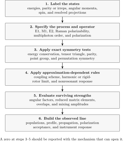
A selection rule is one stage in a spectroscopic forward model. Exact symmetry tests come before approximate coupling rules; a surviving amplitude must still be combined with populations, line shapes, propagation, and the instrument response.

Origin in Matrix Elements

The amplitude is the object being tested

For a weak one-photon process with polarization label $\lambda$, write the transition amplitude as

$$M_{fi}^{(\lambda)} = \langle f| \hat O_{\lambda} |i\rangle.$$

The transition rate or integrated line strength contains $|M_{fi}^{(\lambda)}|^2$ together with frequency, density-of-states, and normalization factors. A selection rule first says

$$M_{fi}^{(\lambda)}=0$$

under specified assumptions. It does not by itself calculate the magnitude when the matrix element is nonzero.

The representation test

Suppose the initial state, final state, and operator transform in representations $\Gamma_i$, $\Gamma_f$, and $\Gamma_O$ of the relevant symmetry group. A necessary condition for a nonzero matrix element is

$$\Gamma_f^* \otimes \Gamma_O \otimes \Gamma_i \supset \Gamma_{\mathrm{ts}},$$

where $\Gamma_{\mathrm{ts}}$ is the totally symmetric representation. For real molecular point-group irreducible representations, the complex conjugation is usually invisible; it remains important in the general rule.

This single test contains parity rules, point-group vibrational activity, and many discrete-symmetry constraints. It is necessary but not always sufficient: the surviving reduced matrix element can vanish dynamically or accidentally.

Rotational factorization

For a spherical tensor component $T_q^{(k)}$, the Wigner–Eckart theorem gives

$$\begin{aligned} &\langle \alpha_fJ_fM_f| T_q^{(k)} |\alpha_iJ_iM_i\rangle \\ &\quad= (-1)^{J_f-M_f} \begin{pmatrix} J_f & k & J_i \\ -M_f & q & M_i \end{pmatrix} \\ &\qquad\times \langle \alpha_fJ_f \|T^{(k)}\| \alpha_iJ_i\rangle. \end{aligned}$$

The $3j$ symbol produces geometric zeros. The reduced matrix element contains the remaining radial, electronic, vibrational, and coupling information. This factorization explains why a line can pass every angular rule yet remain weak.

Rules, line strengths, and observed intensities

A polarization-resolved line strength can be written schematically as

$$S_{i\to f}^{(\lambda)} \propto \left| M_{fi}^{(\lambda)} \right|^2.$$

An observed absorption or emission signal instead has the structure

$$I_{i\to f} \propto p_i S_{i\to f} \mathcal P_{if} \mathcal D_{if},$$

where $p_i$ is an initial population, $\mathcal P_{if}$ represents propagation and profile effects, and $\mathcal D_{if}$ represents detection. Degenerate sublevels may be averaged initially and summed finally. Those operations must be stated before comparing tabulated and measured intensities.

Spectroscopic Operator Ledger

The leading electromagnetic multipoles have different tensor ranks and parities. For multipole order $L$,

$$\begin{aligned} \pi(E L) &= (-1)^L, \\ \pi(M L) &= (-1)^{L+1}. \end{aligned}$$

Process or operator	Effective rank	Operator parity	Immediate consequences
Electric dipole, E1	$1$	odd	Opposite state parity; $\Delta J=0,\pm1$ with $0\leftrightarrow0$ excluded
Magnetic dipole, M1	$1$	even	Same state parity; the same rank-$1$ triangle rule
Electric quadrupole, E2	$2$	even	Same state parity; $
Ordinary nonresonant E1–E1 Raman	$0$ and $2$	even	Same inversion parity; scalar and symmetric-tensor channels

The table gives only rank and parity consequences. Spin, configuration, permutation symmetry, point-group labels, and process-specific cancellations must be checked separately. Resonant Raman scattering, oriented media, magneto-optical terms, and multiphoton processes can require a larger tensor ledger.

Parity Rules

General derivation

Let the states have parity eigenvalues $\pi_i$ and $\pi_f$, and let

$$\hat P\hat O\hat P^{-1} = \pi_O\hat O.$$

Inserting parity transformations into the matrix element gives

$$M_{fi} = \pi_f\pi_O\pi_i M_{fi}.$$

A nonzero amplitude therefore requires

$$\pi_f\pi_O\pi_i = +1.$$

For E1, $\pi_O=-1$, so the states must have opposite parity. For M1 and E2, $\pi_O=+1$, so they must have the same parity.

Atomic parity

Atomic levels are commonly labeled even or odd. In a central-field configuration, the electronic parity is

$$\pi = (-1)^{\sum_a \ell_a}.$$

The familiar one-active-electron E1 rule $\Delta\ell=\pm1$ guarantees a parity change, but it is not the fundamental many-electron rule. Configuration mixing can make the one-electron description ambiguous while exact total parity remains meaningful.

Inversion labels in molecules

For a centrosymmetric molecule, inversion eigenstates carry $g$ or $u$ labels. An E1 operator is ungerade, so

$$g\longleftrightarrow u$$

for electric-dipole transitions. The ordinary polarizability tensor is gerade, so conventional E1–E1 Raman transitions connect states of the same inversion parity.

Parity is not the entire molecular symmetry test. Reflection labels, rotational parity, electronic projections, and nuclear-permutation symmetry can impose additional zeros.

Parity in an external field

A static electric field mixes opposite-parity states. If

$$|\widetilde i\rangle = |i\rangle + \epsilon|a\rangle,$$

where $|a\rangle$ has the opposite parity, a formerly forbidden E1 amplitude can appear at order $\epsilon$. A magnetic field preserves spatial parity but can mix angular-momentum or spin projections. The relevant rule must therefore be applied to the actual field-dressed Hamiltonian, not automatically to its zero-field labels.

Angular Momentum Rules

Tensor rank and projection

The $3j$ symbol in the rotational factorization is nonzero only if

$$|J_i-k| \le J_f \le J_i+k$$

and

$$M_f = M_i+q, \qquad -k\le q\le k.$$

For a rank-$1$ operator this gives

$$\Delta J = 0,\pm1,$$

with $J_i=J_f=0$ excluded by the triangle condition. For E2, rank $2$ allows changes up to two units, again subject to the full triangle inequalities rather than a mnemonic alone.

Electric-dipole atomic rules

For exact atomic levels with total electronic angular momentum $J$ and parity $\pi$, the rigorous E1 core is:

$$\begin{gathered} \pi_f=-\pi_i, \\ \Delta J=0,\pm1, \qquad J_i=J_f=0\ \text{excluded}, \\ \Delta M=q, \qquad q=0,\pm1. \end{gathered}$$

In a good $LS$-coupling limit, one commonly adds

$$\Delta S=0, \qquad \Delta L=0,\pm1,$$

with $L_i=L_f=0$ excluded for E1. These are coupling-scheme rules, not all equally rigorous symmetries of a relativistic many-electron atom.

Polarization and magnetic sublevels

The laboratory spherical component $q$ selects the projection change. Linear polarization along the quantization axis drives the component usually called $\pi$; transverse circular components are called $\sigma^\pm$.

The sign attached to a named helicity depends on the spherical-basis, propagation-direction, and absorption-versus-emission convention. A reliable statement records those conventions and conserves the total projected angular momentum of matter plus radiation. Writing only “$\sigma^+$ means $\Delta M=+1$” without that ledger can hide a sign mismatch between sources.

If the initial ensemble is unpolarized and final magnetic sublevels are not resolved, line strengths require an average and sum:

$$\overline S_{J_i\to J_f} \propto \frac{1}{2J_i+1} \sum_{M_i,M_f,q} \left| \langle f|T_q^{(k)}|i\rangle \right|^2.$$

The resulting Hönl–London or hyperfine factors are quantitative angular weights, not additional yes-or-no rules.

Hyperfine angular momentum

When nuclear spin $I$ couples to electronic $J$ to form $\mathbf F=\mathbf I+\mathbf J$, an electronic E1 operator gives the familiar hyperfine branch rule

$$\Delta F=0,\pm1, \qquad F_i=F_f=0\ \text{excluded},$$

and $\Delta m_F=q$. These conditions do not override a vanishing electronic reduced matrix element. Hyperfine mixing can itself open weak hyperfine-induced transitions, but that is a distinct mechanism.

Spin Selection Rules

Why electric dipole usually preserves spin

In the leading nonrelativistic approximation, the electric-dipole operator

$$\hat{\boldsymbol d} = -e\sum_a \boldsymbol r_a$$

acts on spatial coordinates and is the identity in spin space. If initial and final atomic states factorize into pure total-spin eigenstates, orthogonality gives

$$\langle S_fM_{S,f}|S_iM_{S,i}\rangle = \delta_{S_fS_i} \delta_{M_{S,f}M_{S,i}}.$$

This produces the $\Delta S=0$ E1 rule in pure $LS$ coupling. The same logic supports an approximate spin-multiplicity rule for molecular electronic transitions.

Spin–orbit mixing and intercombination lines

Actual eigenstates need not have pure $S$. Suppose a nominal triplet level contains a small singlet component,

$$|\widetilde t\rangle = \sqrt{1-|\epsilon|^2}|t\rangle + \epsilon|s\rangle.$$

An E1 transition from another singlet then has

$$\langle \widetilde t| \hat{\boldsymbol d} |i_s\rangle \simeq \epsilon^* \langle s| \hat{\boldsymbol d} |i_s\rangle.$$

The borrowed rate is typically proportional to $|\epsilon|^2$ when frequency and phase-space factors are comparable. Such intercombination lines are not violations of quantum mechanics; they measure the failure of pure-spin labels.

When a spin rule changes

Spin selection depends on the operator and Hamiltonian. Magnetic-dipole operators contain spin, spin–orbit and spin–rotation interactions mix labels, hyperfine coupling entangles electronic and nuclear angular momentum, and strong fields can move the system between coupling regimes. State labels should therefore be accompanied by their eigenvector composition when weak lines matter quantitatively.

Vibrational and Rotational Rules

Pure rotational electric-dipole spectra

For the simplest linear rigid rotor in a $^1\Sigma$ electronic state, a permanent body-fixed electric dipole and the rank-$1$ plus parity conditions give

$$\Delta J = \pm1.$$

The $J\to J+1$ branch appears in absorption and the reverse branch in emission. A heteronuclear diatomic such as HCl can possess the required permanent dipole. A homonuclear diatomic such as $\mathrm N_2$ has no permanent electric dipole in its field-free equilibrium state, so its pure rotational E1 spectrum is absent even though rotational energy levels exist.

For a symmetric top, a body-fixed tensor component $p$ and a laboratory component $q$ give the projection rules

$$\Delta K=p, \qquad \Delta M=q.$$

A parallel transition has $p=0$ and hence $\Delta K=0$; a perpendicular transition uses $p=\pm1$ and permits $\Delta K=\pm1$. The rank-$1$ triangle still allows $\Delta J=0,\pm1$ with $0\leftrightarrow0$ excluded, while parity and the detailed rovibronic state can remove some of those branches.

Harmonic vibrational fundamentals

Expand a molecular dipole component in normal coordinates:

$$\begin{aligned} \mu_a(\boldsymbol Q) &= \mu_a^{(0)} + \sum_r \left( \frac{\partial\mu_a}{\partial Q_r} \right)_0 Q_r \\ &\quad+ \frac12 \sum_{r,s} \left( \frac{\partial^2\mu_a} {\partial Q_r\partial Q_s} \right)_0 \\ &\qquad\times Q_rQ_s + \cdots. \end{aligned}$$

In the harmonic and linear-dipole approximations,

$$\langle v_r'|Q_r|v_r\rangle \ne0 \quad\Longrightarrow\quad \Delta v_r=\pm1.$$

For absorption from a low-temperature ground state, the fundamental has $\Delta v_r=+1$. A normal mode is infrared active only if at least one dipole derivative is nonzero. In point-group language, its irrep must transform like one of the vector components $x$, $y$, or $z$.

Overtones and combination bands arise through anharmonic wavefunctions, higher dipole derivatives, mode mixing, or resonance. Calling $\Delta v=\pm1$ an exact molecular law would erase precisely the physics those weak bands reveal.

Rovibrational branches

For a rank-$1$ transition, rotational branches are labeled

$$\begin{array}{c|c} \text{branch} & \Delta J \\ \hline P & -1 \\ Q & 0 \\ R & +1 \end{array}$$

The triangle rule allows all three in a sufficiently general rovibronic transition, except $0\leftrightarrow0$. Additional parity and projection rules decide which survive. A simple $^1\Sigma\leftrightarrow{}^1\Sigma$ diatomic electric-dipole band has $P$ and $R$ branches but no $Q$ branch. It is therefore unsafe to infer “rank $1$ always gives a visible Q branch.”

Permutation symmetry and missing levels

Identical nuclei require the total molecular wavefunction to have the correct exchange symmetry. Electronic, vibrational, rotational, and nuclear-spin factors must be combined before populations are assigned. Alternating rotational levels can be absent or carry different statistical weights.

This is not merely a transition rule between two existing levels. It can be a restriction on which total states exist for a given nuclear-spin species.

Raman Selection Rules

The effective polarizability operator

In ordinary electric-dipole Raman scattering, the leading transition amplitude has the form

$$M_{fi} \propto \boldsymbol e_s^* \mathbin{\boldsymbol\cdot} \boldsymbol\alpha_{fi}(\omega_i) \mathbin{\boldsymbol\cdot} \boldsymbol e_i,$$

where $\boldsymbol e_i$ and $\boldsymbol e_s$ are incident and scattered polarizations and $\boldsymbol\alpha_{fi}$ is a transition polarizability. It encodes the sum over intermediate electronic states. The selection rule is therefore not the one-photon dipole rule applied directly between $|i\rangle$ and $|f\rangle$.

Far from resonance in the ordinary nonmagnetic case, the symmetric polarizability decomposes into rotational ranks $0$ and $2$. Its spatial components transform like

$$x^2, \quad y^2, \quad z^2, \quad xy, \quad xz, \quad yz.$$

Vibrational Raman activity

Expand the polarizability tensor as

$$\alpha_{ab}(\boldsymbol Q) = \alpha_{ab}^{(0)} + \sum_r \left( \frac{\partial\alpha_{ab}} {\partial Q_r} \right)_0 Q_r + \cdots.$$

A fundamental is Raman active if

$$\left( \frac{\partial\alpha_{ab}} {\partial Q_r} \right)_0 \ne0$$

for at least one tensor component sampled by the polarization geometry. In a character table, $\Gamma(Q_r)$ must occur among the quadratic functions. The Raman tensor determines both activity and polarization dependence.

Pure rotational Raman scattering

For a linear molecule with nonzero polarizability anisotropy, the rank-$2$ part gives

$$\Delta J = 0,\pm2.$$

The shifted rotational Raman lines use $\Delta J=\pm2$; the $\Delta J=0$ contribution lies in the elastic Rayleigh channel when no other quantum number changes. Homonuclear diatomics can therefore show rotational Raman spectra even though their permanent-dipole pure rotational E1 spectra vanish.

For a rigid rotor with wavenumber term values

$$F(J) = B J(J+1),$$

the Stokes $J\to J+2$ shift is

$$\Delta\widetilde\nu_J = B(4J+6),$$

so adjacent lines are separated by $4B$ in the rigid-rotor limit.

Infrared–Raman mutual exclusion

In a centrosymmetric molecule, an infrared-active fundamental is ungerade because the dipole operator is odd. An ordinary Raman-active fundamental is gerade because the polarizability is even. Thus, under strict inversion symmetry and the leading electric-dipole models,

no normal mode is both infrared and Raman active.

This mutual-exclusion rule does not say that every gerade mode is Raman active or every ungerade mode is infrared active. The remaining point-group products must still contain an appropriate tensor component. Isotopic substitution, distortion, surfaces, fields, vibronic coupling, resonance, and higher multipoles can weaken the ideal rule.

Resonant and nonlinear Raman caveats

Near an electronic resonance, individual intermediate states and vibronic couplings matter. Antisymmetric tensor contributions, Herzberg–Teller terms, electronic degeneracy, and coherent nonlinear pathways can alter ordinary nonresonant selection rules. Coherent anti-Stokes Raman scattering also has a four-wave-mixing phase-matching and susceptibility tensor, not just a list of normal-mode irreps.

The nonresonant polarizability rule is the correct baseline, not a universal replacement for a process-specific amplitude.

Forbidden but Observable Transitions

Name what is forbidden

“Forbidden line” is shorthand. A complete statement names the leading operator and the symmetry limit, for example:

• E1 parity forbidden;
• E1 spin forbidden in pure $LS$ coupling;
• one-photon E1 forbidden but two-photon allowed;
• infrared inactive but Raman active;
• pure rotational E1 forbidden but collision-induced absorption present; or
• zero-field forbidden but Stark induced.

Different labels predict different strengths, polarization patterns, lifetimes, and responses to control parameters.

Mechanisms that open a line

A nominal zero can acquire intensity through:

1. spin–orbit, configuration, vibronic, Coriolis, or hyperfine mixing;
2. static electric or magnetic fields;
3. symmetry lowering, isotopic substitution, defects, surfaces, or matrices;
4. magnetic-dipole or electric-quadrupole radiation;
5. two-photon, Raman, or other higher-order processes;
6. finite-wavelength corrections beyond the dipole approximation;
7. collision-induced dipoles and transient complexes; or
8. unresolved blending with a nearby allowed transition.

These mechanisms should be tested against polarization, field, pressure, isotope, power, and lifetime dependence rather than inferred from one weak peak alone.

Intensity borrowing

Let an unperturbed transition obey

$$\langle f|\hat O|i_0\rangle = 0,$$

and let a perturbation mix an allowed state $|a\rangle$ into $|i_0\rangle$:

$$|\widetilde i\rangle = |i_0\rangle + \epsilon|a\rangle + O(\epsilon^2).$$

Then

$$\langle f|\hat O|\widetilde i\rangle = \epsilon \langle f|\hat O|a\rangle + O(\epsilon^2),$$

so the borrowed line strength scales as $|\epsilon|^2$ to leading order. An avoided crossing can make $\epsilon$ field dependent, allowing intensity transfer between lines to diagnose the mixing interaction.

Forbidden lines and metastability

When all fast E1 decays are excluded, weak M1, E2, mixed, or multiphoton channels can set the lifetime. The state is then metastable, not stable. Quenching collisions or fields may open much faster decay paths.

A small transition probability does not guarantee a faint observed line. Long-lived states can accumulate population, and low-density astrophysical or trapped-particle environments can suppress collisional quenching. Population kinetics and radiative transfer must be modeled along with the selection rule.

Worked Examples

Atomic E1 hierarchy

Consider three idealized transitions from an even-parity $^1S_0$ level:

1. $^1S_0^{\mathrm e}\to{}^1P_1^{\mathrm o}$ changes parity, satisfies $\Delta J=+1$, $\Delta L=+1$, and $\Delta S=0$. It is E1 allowed by the stated rules.
2. $^1S_0^{\mathrm e}\to{}^3P_1^{\mathrm o}$ passes exact parity and $J$ tests but fails the pure-$LS$ $\Delta S=0$ rule. Spin–orbit mixing can make it an intercombination line.
3. $^1S_0^{\mathrm e}\to{}^1S_0^{\mathrm o}$ changes parity but fails the rank-$1$ $0\leftrightarrow0$ triangle condition. Spin conservation alone cannot rescue the E1 amplitude.

This hierarchy shows why “$\Delta J=0,\pm1$” is not a complete atomic rule.

HCl and nitrogen

HCl can have a permanent body-fixed dipole, so its pure rotational $J\to J+1$ electric-dipole lines are symmetry allowed. Field-free $\mathrm N_2$ is homonuclear and has no permanent electric dipole, so the analogous E1 spectrum is absent.

The polarizability of $\mathrm N_2$ is anisotropic, however. Its pure rotational Raman spectrum has $\Delta J=\pm2$ lines. The molecule has not acquired a permanent dipole; the experiment is probing a different operator.

Carbon dioxide fundamentals

Linear $\mathrm{CO_2}$ has inversion symmetry. Its symmetric stretch is gerade and can be Raman active but is electric-dipole infrared inactive. Its antisymmetric stretch is ungerade and transforms like the molecular-axis dipole component, so it is infrared active and ordinary Raman inactive. The degenerate bend is also ungerade and infrared active in transverse polarization.

The complementary pattern is a direct diagnostic of inversion symmetry. A weak violation can signal symmetry breaking or a process beyond the leading operators, but line overlap and isotopic species must be excluded first.

Practical Assignment Workflow

1. Identify the measured process. Do not apply an E1 absorption rule to a Raman, M1, E2, or multiphoton spectrum.
2. Choose exact eigenstate labels. Separate rigorous parity and total angular momentum from approximate $L$, $S$, $K$, or normal-mode labels.
3. Write the operator. Record tensor rank, parity, body-fixed component, and spin dependence.
4. Apply exact symmetries first. Use parity, angular momentum, point-group, and permutation tests.
5. Apply coupling-limit rules second. State the assumed $LS$, Hund’s-case, rigid-rotor, harmonic, or nonresonant Raman approximation.
6. Compute angular factors. A branch that survives can still have a small Clebsch–Gordan, Hönl–London, or Raman-tensor weight.
7. Evaluate the reduced matrix element. Include radial overlap, Franck–Condon factors, dipole derivatives, or polarizability derivatives.
8. Build the observable. Add populations, degeneracies, line shapes, optical depth, polarization acceptance, and instrument response.
9. Challenge weak lines. Test field, pressure, isotope, power, and temperature scaling to identify the opening mechanism.
10. Report the rule’s status. Say exact, approximate, or propensity, and name the Hamiltonian and operator model.

Common Mistakes

Applying a rule without naming the operator

E1, M1, E2, infrared, and Raman transitions obey different parity and tensor rules. “Forbidden” without an operator is incomplete.

Treating energy conservation as a selection rule

Resonance identifies a possible energy difference. It does not make the coupling matrix element nonzero.

Treating ΔS = 0 as an exact relativistic law

It is exact only in the stated spin-independent, pure-spin approximation. Spin–orbit mixing produces intercombination intensity.

Forgetting the 0 ↔ 0 exception

A rank-$1$ operator cannot connect two $J=0$ states even though the mnemonic $\Delta J=0$ seems to permit it.

Confusing space-fixed and body-fixed projections

$M$ refers to a laboratory quantization axis; $K$, $\Lambda$, or $\Omega$ refer to molecule-fixed projections. Polarization selects the former, while parallel and perpendicular transition moments constrain the latter.

Calling every Δv > 1 line forbidden by symmetry

The harmonic-plus-linear-dipole rule suppresses overtones. Anharmonicity and higher dipole derivatives make them generically weak rather than absolutely absent.

Saying homonuclear molecules have no rotational spectrum

They lack a permanent-dipole pure rotational E1 spectrum, but may have rotational Raman, quadrupole, magnetic, or collision-induced spectra.

Overstating infrared–Raman mutual exclusion

It requires inversion symmetry and leading E1 infrared and ordinary E1–E1 Raman operators. It also does not guarantee that every mode is active in one of the two channels.

Equating allowed with strong

Angular rules do not determine radial overlap, Franck–Condon factors, populations, or destructive interference in the reduced matrix element.

Inferring new physics from one forbidden peak

Blends, isotopologues, fields, collisions, detector artifacts, and known mixing mechanisms should be tested first.

Key Takeaways

1. A selection rule is a matrix-element zero tied to a specific operator, symmetry limit, and set of state labels.
2. Exact rules, coupling-scheme approximations, and propensity rules must be reported separately.
3. Parity requires $\pi_f\pi_O\pi_i=+1$; E1 changes parity, while M1 and E2 preserve it.
4. A rank-$k$ tensor obeys angular-momentum triangle and projection rules; polarization selects its component $q$.
5. The E1 $\Delta S=0$ rule reflects a spin-independent operator acting on pure-spin states and is weakened by spin mixing.
6. Rotational and vibrational rules require permanent or transition moments, body-fixed projections, molecular symmetry, and nuclear statistics in addition to $\Delta J$ or $\Delta v$ mnemonics.
7. Raman activity is governed by a transition polarizability, not by the direct one-photon dipole matrix element.
8. A forbidden but observed line identifies an omitted interaction or a different process; its scaling and polarization should reveal which one.

Exercises

Exercise 1: Audit four atomic E1 candidates

In a pure $LS$-coupling description, classify the following proposed E1 transitions by the first rule that fails:

1. $^2S_{1/2}^{\mathrm e}\to{}^2P_{3/2}^{\mathrm o}$;
2. $^1S_0^{\mathrm e}\to{}^3P_1^{\mathrm o}$;
3. $J=0$ even $\to J=0$ odd; and
4. $J=1$ even $\to J=1$ even.

Solution

1. The first transition changes parity, has $\Delta J=+1$, and preserves spin multiplicity. It is E1 allowed by the listed rules.
2. The second changes parity and satisfies the rank-$1$ $J$ rule, but $\Delta S\ne0$. It is spin forbidden in pure $LS$ coupling and can borrow intensity through spin–orbit mixing.
3. The third changes parity but fails the $J=0\leftrightarrow0$ rank-$1$ triangle condition.
4. The fourth satisfies $\Delta J=0$ and is not a $0\leftrightarrow0$ transition, but it fails E1 parity because both levels are even. An M1 or E2 channel would require its own additional tests.

Exercise 2: Polarization from a scalar state

An atom begins in $J_i=0$, $M_i=0$ and is driven to $J_f=1$. Which final $M_f$ is addressed by each spherical E1 component $q=-1,0,+1$? Why is a helicity name alone insufficient to fix the sign in every source?

Solution

The projection rule gives

$$M_f = M_i+q = q.$$

Thus $q=-1,0,+1$ addresses $M_f=-1,0,+1$, respectively. The labels $\sigma^+$ and $\sigma^-$ depend on the propagation direction, spherical basis, and whether the matter or photon projection change is being named. Those conventions must accompany the helicity label.

Exercise 3: Hyperfine branches

Which of the branches $F_i=0\to F_f=0$, $0\to1$, $1\to0$, and $1\to2$ pass the rank-$1$ hyperfine angular rule? Does passing it prove that the electronic E1 amplitude is nonzero?

Solution

The rank-$1$ rule permits $\Delta F=0,\pm1$ but excludes $0\leftrightarrow0$. Therefore $0\to1$, $1\to0$, and $1\to2$ pass, while $0\to0$ fails.

Passing the $F$ rule is only necessary. The electronic reduced matrix element can still vanish by parity, the electronic $J$ rule, configuration symmetry, or another exact condition.

Exercise 4: Fundamental and overtone amplitudes

For one harmonic normal coordinate $Q$, keep

$$\mu(Q) = \mu_0 + \mu'Q + \frac12\mu''Q^2.$$

Which term first drives $v=0\to1$, and which first drives $v=0\to2$ in the harmonic basis?

Solution

Writing $Q\propto a+a^\dagger$, the linear term has

$$\langle1|Q|0\rangle \ne0,$$

so $\mu'Q$ drives the fundamental. Since $Q^2$ contains $(a^\dagger)^2$, the quadratic term has

$$\langle2|Q^2|0\rangle \ne0,$$

and first drives the overtone in this truncated electrical-anharmonicity model. Anharmonic eigenstates can also give $\langle2|Q|0\rangle\ne0$ after state mixing.

Exercise 5: HCl versus nitrogen

Explain why HCl can show a $J=0\to1$ microwave absorption line while $\mathrm N_2$ does not, and why $\mathrm N_2$ can nevertheless show a $J=0\to2$ rotational Raman line.

Solution

HCl can possess a permanent electric dipole, so its rank-$1$ pure rotational E1 matrix element is nonzero and $\Delta J=+1$ is allowed. In field-free $\mathrm N_2$, inversion and nuclear symmetry force the permanent electric dipole to vanish, so the corresponding E1 line is absent.

The polarizability of $\mathrm N_2$ is anisotropic. The rank-$2$ component of the Raman polarizability permits $\Delta J=+2$, so $J=0\to2$ can appear in a Raman spectrum without a permanent dipole.

Exercise 6: Prove mutual exclusion

Use inversion parity to show that a normal-mode fundamental of a centrosymmetric molecule cannot be both electric-dipole infrared active and ordinary E1–E1 Raman active.

Solution

The vibrational ground state is gerade. The electric dipole is ungerade, so the matrix element

$$\langle1_r|\mu_a|0\rangle$$

can be nonzero only if the one-quantum mode is ungerade. The ordinary polarizability tensor is gerade, so

$$\langle1_r|\alpha_{ab}|0\rangle$$

can be nonzero only if the mode is gerade. One mode cannot have both inversion parities, so the two activities are mutually exclusive under the stated approximations.

Exercise 7: Rotational Raman spacing

A linear rigid rotor has $F(J)=BJ(J+1)$ in wavenumber units. Derive the Stokes $J\to J+2$ Raman shift and the spacing between adjacent shifted lines.

Solution

The shift is

$$\begin{aligned} \Delta\widetilde\nu_J &= F(J+2)-F(J) \\ &= B\left[ (J+2)(J+3)-J(J+1) \right] \\ &= B(4J+6). \end{aligned}$$

Therefore

$$\Delta\widetilde\nu_{J+1} - \Delta\widetilde\nu_J = 4B.$$

Nuclear-spin statistics can remove some initial $J$ values, changing the observed alternation without changing this rigid-rotor spacing formula.

Exercise 8: Estimate borrowed intensity

A forbidden state contains an allowed-state amplitude $|\epsilon|=2.0\times10^{-2}$. A comparable fully allowed transition has $A=1.0\times10^8\ \mathrm{s}^{-1}$. Neglect frequency and angular-factor differences. Estimate the borrowed rate and lifetime if this is the only decay channel.

Solution

The rate scales as $|\epsilon|^2$:

$$\begin{aligned} A_{\mathrm{borrowed}} &\simeq |\epsilon|^2 A_{\mathrm{allowed}} \\ &= (2.0\times10^{-2})^2 \\ &\quad\times (1.0\times10^8\ \mathrm{s}^{-1}) \\ &= 4.0\times10^4\ \mathrm{s}^{-1}. \end{aligned}$$

If no other decay exists,

$$\tau = \frac{1}{A_{\mathrm{borrowed}}} = 25\ \mu\mathrm s.$$

In a real system, all radiative, nonradiative, and quenching channels must be summed before identifying the measured lifetime.

Cross-Links

• Spectroscopy
• Transition Rates
• Oscillator Strengths
• Absorption and Emission
• Line Shapes and Broadening
• Rotational Spectroscopy
• Vibrational Spectroscopy
• Infrared Spectroscopy
• Raman Spectroscopy
• Electronic Spectroscopy
• Fluorescence and Phosphorescence
• Atomic Selection Rules
• Molecular Symmetry
• Vibrations of Diatomics
• Rovibrational Coupling
• Selection Rules
• Wigner–Eckart Theorem
• Dipole Transitions
• Multipole Operators
• Selection Rules in Transition Rates
• Selection Rule Tables for a compact operator-by-operator lookup

References

• International Union of Pure and Applied Chemistry, “selection rule”, Compendium of Chemical Terminology, 5th ed., online version 5.0.0, 2025.
• W. C. Martin, W. L. Wiese, and A. Kramida, “Spectral Lines: Selection Rules, Intensities, Transition Probabilities, Values, and Line Strengths”, NIST Atomic Spectroscopy: A Compendium of Basic Ideas, Notation, Data, and Formulas, updated 2025, accessed 2026-07-22.
• NIST Atomic Spectra Database, Spectral Lines Help, Standard Reference Database 78, accessed 2026-07-22.
• R. N. Zare, Angular Momentum: Understanding Spatial Aspects in Chemistry and Physics, Wiley, 1988.
• I. I. Sobelman, Atomic Spectra and Radiative Transitions, 2nd ed., Springer, 1992, doi:10.1007/978-3-642-76709-8.
• P. F. Bernath, Spectra of Atoms and Molecules, 5th ed., Oxford University Press, 2025, doi:10.1093/oso/9780197754498.001.0001.
• P. R. Bunker and P. Jensen, Molecular Symmetry and Spectroscopy, 2nd ed., NRC Research Press, 2006.
• J. M. Brown and A. Carrington, Rotational Spectroscopy of Diatomic Molecules, Cambridge University Press, 2003, doi:10.1017/CBO9780511814808.
• D. A. Long, The Raman Effect: A Unified Treatment of the Theory of Raman Scattering by Molecules, Wiley, 2002, doi:10.1002/0470845767.
• D. C. Harris and M. D. Bertolucci, Symmetry and Spectroscopy: An Introduction to Vibrational and Electronic Spectroscopy, Dover, 1989.