Raman Spectroscopy

Raman spectroscopy measures inelastic scattering in which incident and scattered photons differ in energy because the material changes its internal state. In ordinary molecular Raman spectroscopy, the dominant off-resonant signal is controlled by how the electric polarizability changes during a rotation or vibration. This is a different coupling from direct infrared absorption, which is controlled by the electric dipole moment.

The experimental inference chain is

$$\begin{gathered} \text{laser and prepared sample} \\ \downarrow \\ \text{elastic and inelastic scattering} \\ \downarrow \\ \begin{matrix} \text{Rayleigh rejection, dispersion,}\\ \text{polarization analysis} \end{matrix} \\ \downarrow \\ \text{Raman shifts and line areas} \\ \downarrow \\ \begin{matrix} \text{state, symmetry, temperature,}\\ \text{or composition inference} \end{matrix}. \end{gathered}$$

Each arrow carries assumptions. A peak position can identify an energy difference, but its observed height also depends on the excitation frequency, Raman tensor, population, optical geometry, line shape, instrument response, and sample stability. Raman spectra are information-rich precisely because the scattering amplitude retains all of these dependencies.

Canonical Scope

This page owns the ordinary spontaneous Raman workflow for:

• defining Raman shift and distinguishing Rayleigh, Stokes, and anti-Stokes scattering;
• connecting an induced dipole and polarizability derivative to vibrational sidebands;
• deriving the transition polarizability from the Kramers–Heisenberg–Dirac amplitude;
• applying Raman-tensor, polarization, inversion, and rotational selection rules;
• interpreting depolarization ratios and Stokes/anti-Stokes ratios;
• recognizing pure rotational and vibration–rotation Raman structure;
• explaining what changes near electronic resonance; and
• separating molecular response from laser, collection, calibration, fluorescence, and heating effects.

Nearby pages retain their own canonical roles:

• Vibrational Spectroscopy owns normal-mode assignments, anharmonic term values, overtones, combinations, and force-field inference.
• Normal Modes of Polyatomics derives the mass-weighted Hessian and normal coordinates.
• Vibrational Spectra Computation supplies an executable CO$_2$ symmetry benchmark and explains why a Raman intensity requires a polarizability surface rather than a frequency alone.
• Selection Rules in Spectroscopy owns the cross-method hierarchy of exact, approximate, and propensity rules.
• Infrared Spectroscopy owns dipole-derivative activity and infrared sampling methods.
• Rotational Spectroscopy owns permanent-dipole rotational absorption and the extraction of rotational constants.
• Transition Rates owns general perturbative rate logic and normalization conventions.

The present page specializes those ingredients to inelastic optical scattering. Surface-enhanced, coherent, time-resolved, and X-ray Raman methods use related language but require additional electromagnetic or nonlinear response models.

Raman Shift and Energy Conservation

Incident, scattered, and material frequencies

Let the incident laser have angular frequency $\omega_L$ and the detected photon have angular frequency $\omega_s$. If the material begins in $|i\rangle$ and ends in $|f\rangle$, energy conservation gives

$$E_i+\hbar\omega_L = E_f+\hbar\omega_s.$$

Define the material transition frequency by

$$\Omega_{fi} = \frac{E_f-E_i}{\hbar}.$$

Then

$$\omega_s = \omega_L-\Omega_{fi}.$$

Three cases follow:

Process	Material change	Scattered photon
Rayleigh	$E_f=E_i$	$\omega_s=\omega_L$
Stokes Raman	$E_f>E_i$	$\omega_s<\omega_L$
Anti-Stokes Raman	$E_f<E_i$	$\omega_s>\omega_L$

The labels describe the net initial and final states. They do not assert that the system occupies a stationary level at the laser photon energy during the scattering event.

Wavenumber-shift convention

Spectra are commonly plotted against the Raman wavenumber shift

$$\Delta\widetilde\nu = \widetilde\nu_L-\widetilde\nu_s,$$

where the wavenumbers refer to vacuum. With this IUPAC convention,

$$\Delta\widetilde\nu = \frac{E_f-E_i}{hc}.$$

Thus Stokes shifts are positive and anti-Stokes shifts are negative. Some instruments plot the anti-Stokes side against a positive shift magnitude, so the axis definition must accompany the data.

For a fixed material transition, the Raman shift is approximately independent of laser frequency even though the detected wavelength is not. Since

$$\widetilde\nu_s = \widetilde\nu_L-\Delta\widetilde\nu,$$

changing the laser changes the scattered wavelength and the optical response of every filter, grating, and detector in the experiment.

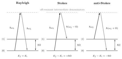
Energy bookkeeping for three scattering channels. The gray dashed intermediate guides represent off-resonant energy denominators, not stationary molecular eigenstates. In Stokes scattering the material gains $\hbar\Omega$; in anti-Stokes scattering it loses $\hbar\Omega$.

Raman shift is not fluorescence wavelength

An elementary diagnostic is to repeat a measurement with another excitation wavelength:

• an ordinary Raman feature follows the laser while retaining approximately the same Raman shift;
• an ordinary fluorescence band is more naturally organized around an emission energy set by real electronic states; and
• resonance Raman, reabsorption, energy transfer, hot luminescence, and dispersive backgrounds can complicate this contrast.

Laser-shift testing is evidence, not a universal classifier. Time dependence, polarization, linewidth, power scaling, and sample chemistry provide independent checks.

Polarizability and Induced Dipoles

Linear optical response

For an applied electric field $\mathbf E(t)$, the induced molecular dipole is, to leading order,

$$p_a(t) = \sum_b \alpha_{ab}(\mathbf Q;\omega_L) E_b(t).$$

The dynamic polarizability tensor $\boldsymbol\alpha(\mathbf Q;\omega_L)$ depends on the nuclear geometry $\mathbf Q$ and the optical frequency. Far from absorption resonances in a transparent, nonmagnetic system it can often be treated as approximately real and symmetric. Near resonance or in an absorbing sample it is generally complex and strongly frequency dependent.

For normal coordinates $Q_k$ near equilibrium, fix $\omega_L$, suppress it temporarily in the coefficient labels, and expand

$$\begin{aligned} \alpha_{ab}(\mathbf Q) ={}& \alpha_{ab}^{(e)} \\ &+ \sum_k R_{ab}^{(k)}Q_k \\ &+ \frac12 \sum_{kl} R_{ab}^{(kl)}Q_kQ_l +\cdots, \end{aligned}$$

where

$$\begin{aligned} R_{ab}^{(k)} &\equiv \left( \frac{\partial\alpha_{ab}} {\partial Q_k} \right)_e, \\ R_{ab}^{(kl)} &\equiv \left( \frac{\partial^2\alpha_{ab}} {\partial Q_k\partial Q_l} \right)_e. \end{aligned}$$

$\mathbf R^{(k)}$ is the first-order Raman tensor of mode $k$ in the off-resonant Placzek approximation.

Classical sideband derivation

Take one linearly polarized field and one classical normal coordinate,

$$\begin{aligned} E(t)&=E_0\cos\omega_L t, \\ Q(t)&=Q_0\cos\Omega t. \end{aligned}$$

Keeping one scalar polarizability component,

$$\alpha(Q) \simeq \alpha_e+\alpha'Q,$$

the induced dipole becomes

$$\begin{aligned} p(t) ={}& \alpha_eE_0\cos\omega_L t \\ &+ \frac{\alpha'Q_0E_0}{2} \cos(\omega_L-\Omega)t \\ &+ \frac{\alpha'Q_0E_0}{2} \cos(\omega_L+\Omega)t. \end{aligned}$$

An oscillating dipole radiates. The first term produces elastic Rayleigh scattering; the other two produce frequency-shifted sidebands. This argument gets the frequencies and the leading derivative rule right:

$$\alpha'\ne0 \quad\Longrightarrow\quad \text{Raman-active motion}.$$

It does not by itself explain spontaneous scattering from a vibrational ground state, the Bose population factors, single-photon statistics, or the detailed interference among electronic intermediate states. Those require a quantum description.

A permanent dipole is not required

Raman activity asks whether the electron cloud’s deformability changes along the motion. A molecule can therefore have:

• no permanent dipole but a nonzero polarizability anisotropy;
• an infrared-inactive vibration with a nonzero polarizability derivative; or
• a permanent dipole while a particular polarizability derivative vanishes.

Homonuclear diatomics such as $\mathrm N_2$ illustrate the first case. Their permanent-dipole pure rotational absorption is absent, but their anisotropic polarizability permits rotational Raman scattering.

Quantum Scattering Amplitude

Transition polarizability

In the electric-dipole approximation, the scattering amplitude for incident polarization $\boldsymbol e_L$ and detected polarization $\boldsymbol e_s$ has the form

$$\mathcal M_{fi} \propto \boldsymbol e_s^* \mathbin{\boldsymbol\cdot} \boldsymbol\alpha_{fi}(\omega_L) \mathbin{\boldsymbol\cdot} \boldsymbol e_L.$$

Write electric-dipole matrix elements as

$$\mu_{mn}^{a} = \langle m|\hat\mu_a|n\rangle.$$

One common Kramers–Heisenberg–Dirac convention introduces

$$\begin{aligned} D_n^{(-)} &= E_n-E_i-\hbar\omega_L -\frac{i\Gamma_n}{2}, \\ D_n^{(+)} &= E_n-E_i+\hbar\omega_s +\frac{i\Gamma_n}{2}, \end{aligned}$$

and writes

$$\begin{aligned} \alpha_{fi}^{ab}(\omega_L) ={}& \sum_n \frac{\mu_{fn}^{a}\mu_{ni}^{b}} {D_n^{(-)}} \\ &+ \sum_n \frac{\mu_{fn}^{b}\mu_{ni}^{a}} {D_n^{(+)}}. \end{aligned}$$

The two sums are the two time orderings of the dipole interactions. $\Gamma_n$ represents finite intermediate-state width in this phenomenological form. Overall signs and damping conventions vary across sources, but the physical content does not: amplitudes from all intermediate states and both orderings add coherently before the modulus is squared.

The intermediate label $n$ runs over actual eigenstates used in the resolution of identity. A “virtual state” in a level diagram is shorthand for this off-shell sum and its energy denominators; it is not an additional stationary molecular level with a measurable lifetime.

Differential cross-section structure

Suppressing unit-system and normalization constants, spontaneous electric dipole Raman scattering has the structure

$$\frac{d\sigma_{fi}} {d\Omega_s} \propto \omega_s^4 \left| \boldsymbol e_s^* \mathbin{\boldsymbol\cdot} \boldsymbol\alpha_{fi} \mathbin{\boldsymbol\cdot} \boldsymbol e_L \right|^2.$$

The familiar fourth-power factor is only one part of the laser dependence. The transition polarizability itself is dynamic, and collection optics and detector responsivity change with $\omega_s$. Raw intensities acquired with different lasers are therefore not made comparable by a wavelength-to-the- fourth correction alone.

Placzek limit

Far from electronic resonance, the electronic response can vary smoothly with the nuclear coordinates. Under Born–Oppenheimer and Placzek approximations, the vibronic transition polarizability reduces schematically to

$$\alpha_{v'v}^{ab} \simeq \left\langle v'\right| \alpha_{ab}(\mathbf Q;\omega_L) \left|v\right\rangle.$$

For a harmonic fundamental of mode $k$,

$$\begin{aligned} \alpha_{1_k0}^{ab} &\simeq R_{ab}^{(k)} \left\langle1_k\right| Q_k \left|0_k\right\rangle \\ &= R_{ab}^{(k)} \sqrt{\frac{\hbar}{2\Omega_k}}. \end{aligned}$$

The leading Raman-activity condition is therefore

$$R_{ab}^{(k)}\ne0$$

for at least one tensor component admitted by the measurement geometry. Higher polarizability derivatives, anharmonic state mixing, vibronic coupling, and resonance effects produce overtone and combination intensity beyond this leading rule.

Stokes and Anti-Stokes Scattering

Harmonic-oscillator matrix elements

For one normal mode,

$$Q = \sqrt{\frac{\hbar}{2\Omega}} \left(a+a^\dagger\right).$$

The adjacent-level matrix elements are

$$\begin{aligned} \left|\langle v+1|Q|v\rangle\right|^2 &= \frac{\hbar}{2\Omega}(v+1), \\ \left|\langle v-1|Q|v\rangle\right|^2 &= \frac{\hbar}{2\Omega}v. \end{aligned}$$

Stokes scattering creates one vibrational quantum and carries the factor $v+1$. Anti-Stokes scattering removes one and requires an initial excitation, giving the factor $v$.

Thermal occupation and intensity ratio

At thermal equilibrium the mean harmonic occupation is

$$\bar n = \frac{1} {\exp(\hbar\Omega/k_{\mathrm B}T)-1}.$$

Under the same collection geometry and a slowly varying transition polarizability,

$$\begin{aligned} I_{\mathrm S} &\propto \omega_{\mathrm S}^4(\bar n+1), \\ I_{\mathrm{AS}} &\propto \omega_{\mathrm{AS}}^4\bar n. \end{aligned}$$

Hence

$$\frac{I_{\mathrm{AS}}} {I_{\mathrm S}} = \left( \frac{\omega_L+\Omega} {\omega_L-\Omega} \right)^4 \exp\left( -\frac{\hbar\Omega} {k_{\mathrm B}T} \right).$$

In wavenumber units, use

$$\frac{\hbar\Omega}{k_{\mathrm B}T} = \frac{hc\Delta\widetilde\nu} {k_{\mathrm B}T}.$$

For a $1000\ \mathrm{cm}^{-1}$ mode, 532 nm excitation, and $T=300\ \mathrm K$, the Boltzmann factor is about $8.26\times10^{-3}$ and the fourth-power factor is about $1.53$, giving

$$\frac{I_{\mathrm{AS}}}{I_{\mathrm S}} \approx 1.27\times10^{-2}.$$

This explains why room-temperature vibrational Raman spectra are commonly recorded on the Stokes side.

Raman thermometry requires calibration

Solving the ratio for temperature gives

$$T = \frac{hc\Delta\widetilde\nu}{k_{\mathrm B}} \left[ \ln\left( \frac{I_{\mathrm S}}{I_{\mathrm{AS}}} \frac{\omega_{\mathrm{AS}}^4} {\omega_{\mathrm S}^4} \right) \right]^{-1}.$$

That expression is valid only after accounting for:

1. wavelength-dependent throughput and detector response;
2. different Rayleigh-filter transmission on the two sides;
3. polarization acceptance and collection geometry;
4. background and baseline subtraction;
5. reabsorption or self-absorption;
6. resonance-dependent tensor changes;
7. overlapping bands and line-shape integration; and
8. nonequilibrium mode populations or laser heating.

A Stokes/anti-Stokes temperature is a mode-population temperature under a model. Agreement among several modes, laser powers, and independent thermometers is stronger evidence for thermal equilibrium.

Raman Selection Rules

Tensor representation test

For a normal coordinate $Q_k$, the first-order Raman tensor transforms as the symmetric second-rank Cartesian products. The matrix-element test can be written as

$$\Gamma(v_f) \otimes \Gamma(\alpha_{ab}) \otimes \Gamma(v_i) \supset \Gamma_{\mathrm{tot.sym.}}.$$

From a nondegenerate totally symmetric vibrational ground state, a fundamental is Raman active when

$$\Gamma(Q_k) \subset \Gamma_{\mathrm{sym}}^{(2)},$$

where the right side is spanned by

$$x^2,\ y^2,\ z^2,\ xy,\ xz,\ yz.$$

This is the character-table version of $R_{ab}^{(k)}\ne0$. It determines which tensor elements may survive, not how large they are.

Raman tensors and laboratory polarization

For a fixed molecular or crystal orientation, the idealized mode intensity is

$$I_k \propto \left| \boldsymbol e_s^* \mathbin{\boldsymbol\cdot} \mathbf R^{(k)} \mathbin{\boldsymbol\cdot} \boldsymbol e_L \right|^2.$$

As an example, in the standard $C_{2v}$ convention with $z$ as the twofold axis, representative symmetric Raman tensors are

$$\begin{aligned} \mathbf R(A_1) &= \begin{pmatrix} a&0&0\\ 0&b&0\\ 0&0&c \end{pmatrix}, \\ \mathbf R(B_1) &= \begin{pmatrix} 0&0&d\\ 0&0&0\\ d&0&0 \end{pmatrix}, \\ \mathbf R(B_2) &= \begin{pmatrix} 0&0&0\\ 0&0&e\\ 0&e&0 \end{pmatrix}. \end{aligned}$$

The $A_2$ tensor has symmetric $xy$ and $yx$ entries. Rotating the sample rotates these tensors into the laboratory frame. A missing line in one polarization geometry can therefore be a geometric zero rather than a mode that is inactive in every geometry.

Isotropic samples and depolarization

For a real symmetric mode tensor, define its isotropic invariant

$$\overline R = \frac13 \left( R_{xx}+R_{yy}+R_{zz} \right),$$

and anisotropy invariant

$$\begin{aligned} \gamma^2 ={}& \frac12(R_{xx}-R_{yy})^2 \\ &+ \frac12(R_{yy}-R_{zz})^2 \\ &+ \frac12(R_{zz}-R_{xx})^2 \\ &+ 3\left( R_{xy}^2+R_{yz}^2+R_{zx}^2 \right). \end{aligned}$$

In the standard ideal 90-degree experiment with linearly polarized excitation,

$$\begin{aligned} I_\parallel &\propto 45\overline R^2+4\gamma^2, \\ I_\perp &\propto 3\gamma^2. \end{aligned}$$

The depolarization ratio is

$$\rho \equiv \frac{I_\perp}{I_\parallel} = \frac{3\gamma^2} {45\overline R^2+4\gamma^2}.$$

For ordinary nonresonant Raman scattering in an isotropic sample, $\rho\le3/4$ for a totally symmetric vibration and $\rho=3/4$ for a nontotally symmetric vibration under the ideal assumptions. A totally symmetric band need not have $\rho=0$; anisotropy can make it partially depolarized.

Computational chemistry programs often report the orientationally averaged Raman activity

$$S_k = 45\overline R_k^2+7\gamma_k^2.$$

$S_k$ is not a raw experimental peak height. Converting it to a simulated spectrum requires excitation frequency, scattered-frequency factors, population, line shape, temperature, and a stated differential or integrated intensity convention.

Infrared–Raman complementarity

The leading activity tests are

$$\begin{aligned} \text{infrared:}\quad& \left( \frac{\partial\mu_a}{\partial Q_k} \right)_e \ne0, \\ \text{Raman:}\quad& \left( \frac{\partial\alpha_{ab}}{\partial Q_k} \right)_e \ne0. \end{aligned}$$

Feature	Infrared absorption	Ordinary Raman scattering
Leading material operator	Dipole derivative	Polarizability derivative
Optical process	One incident photon absorbed	Incident photon scattered into another mode
Tensor character	Vector	Symmetric rank $0$ and $2$ parts
Homonuclear diatomic rotation	Permanent-dipole E1 inactive	Can be active through anisotropy
Common experimental challenge	Optical propagation and saturation	Weak signal, Rayleigh rejection, fluorescence

In a centrosymmetric molecule, the dipole operator is ungerade while the ordinary polarizability is gerade. Therefore a first-order fundamental cannot be both electric-dipole infrared active and ordinary Raman active. This mutual-exclusion rule requires exact inversion symmetry and the stated leading operators. It does not say every mode must appear in one spectrum, and it can be weakened by symmetry lowering, isotopic composition, surfaces, fields, resonance mechanisms, or higher multipoles.

For linear $\mathrm{CO_2}$, the gerade symmetric stretch is Raman active and infrared inactive at leading order. The ungerade bend and antisymmetric stretch are infrared active and ordinary Raman inactive. Water lacks inversion symmetry, so its fundamentals can be active in both methods.

Harmonic and anharmonic rules

With a linear polarizability expansion and harmonic states,

$$\Delta v_k = \pm1$$

is the leading one-mode rule. A quadratic derivative can produce overtones and combinations through matrix elements such as

$$\langle2_k|Q_k^2|0_k\rangle\ne0$$

and

$$\langle1_k1_l|Q_kQ_l|0\rangle\ne0.$$

Anharmonic eigenstate mixing can also make a linear polarizability term contribute to nominal overtones. Calling every $\Delta v>1$ feature “forbidden” hides the actual approximation that suppresses it.

Rotational Raman Spectroscopy

Polarizability anisotropy

For a linear molecule, define body-fixed components parallel and perpendicular to the molecular axis. Its polarizability anisotropy is

$$\Delta\alpha = \alpha_\parallel-\alpha_\perp.$$

If $\Delta\alpha=0$, reorientation does not modulate the induced dipole and shifted pure rotational Raman scattering vanishes in the leading model. If $\Delta\alpha\ne0$, the rank-$2$ polarizability channel permits

$$\Delta J = 0,\pm2.$$

For pure rotational Raman scattering, $\Delta J=0$ belongs to the elastic channel; shifted lines use $\Delta J=\pm2$.

Rigid-rotor line positions

For term values

$$F(J) = BJ(J+1),$$

the Stokes transition $J\to J+2$ has shift

$$\begin{aligned} \Delta\widetilde\nu_J^{(\mathrm S)} &= F(J+2)-F(J) \\ &= B(4J+6). \end{aligned}$$

The first line, from $J=0$, occurs at $6B$, and adjacent allowed initial $J$ values give a spacing of

$$\Delta\widetilde\nu_{J+1}^{(\mathrm S)} - \Delta\widetilde\nu_J^{(\mathrm S)} = 4B.$$

The anti-Stokes transition $J\to J-2$ has shift magnitude

$$\left| \Delta\widetilde\nu_J^{(\mathrm{AS})} \right| = B(4J-2), \qquad J\ge2.$$

Centrifugal distortion makes the spacings nonuniform. Nuclear-spin statistics can suppress alternating initial levels or change their statistical weights. Populations, degeneracies, Placzek–Teller factors, and the $\omega_s^4$ factor determine line strengths.

Nitrogen example

Taking $B\approx1.99\ \mathrm{cm}^{-1}$ for a rigid-rotor estimate of $\mathrm N_2$, the first two Stokes shifts are

$$\begin{aligned} J=0\to2:\quad& 6B \approx 11.94\ \mathrm{cm}^{-1}, \\ J=1\to3:\quad& 10B \approx 19.90\ \mathrm{cm}^{-1}. \end{aligned}$$

Their separation is $4B\approx7.96\ \mathrm{cm}^{-1}$. A real spectrum must also include centrifugal distortion and the nuclear-spin statistical pattern of the isotopologue.

Vibration–rotation Raman branches

For a linear molecule, a Raman-active vibrational transition can carry

$$\Delta J = 0,\pm2,$$

giving O, Q, and S branches in a common convention:

Branch	Rotational change
O	$\Delta J=-2$
Q	$\Delta J=0$
S	$\Delta J=+2$

If the lower and upper vibrational states have constants $B_0$ and $B_1$, the simple branch shifts are

$$\begin{aligned} \Delta\widetilde\nu_{\mathrm Q}(J) &= \widetilde\nu_0 +(B_1-B_0)J(J+1), \\ \Delta\widetilde\nu_{\mathrm S}(J) &= \widetilde\nu_0 +B_1(J+2)(J+3) \\ &\quad -B_0J(J+1), \\ \Delta\widetilde\nu_{\mathrm O}(J) &= \widetilde\nu_0 +B_1(J-2)(J-1) \\ &\quad -B_0J(J+1). \end{aligned}$$

Electronic symmetry, vibrational angular momentum, polarization, and nuclear statistics can refine this simple branch picture. The detailed molecular Hamiltonian and Coriolis structure remain in Rovibrational Coupling.

Resonance Raman Spectroscopy

Near an electronic transition

When $\hbar\omega_L$ approaches a real electronic or vibronic transition, one or more denominators

$$D_n^{(-)} = E_n-E_i-\hbar\omega_L -\frac{i\Gamma_n}{2}$$

become small. The scattering can be enhanced by many orders of magnitude, but the off-resonant approximation also becomes less reliable. The measured tensor can become complex, excitation-frequency dependent, and sensitive to individual intermediate states.

Resonance Raman spectroscopy is therefore selective rather than merely stronger. Modes coupled to the resonant chromophore or electronic excitation can be enhanced far more than spectator modes.

Franck–Condon and vibronic mechanisms

In Albrecht’s organization of molecular resonance Raman amplitudes:

• the A term is associated with Franck–Condon structure and displacement of an allowed excited-state potential surface;
• the B and C terms involve vibronic, or Herzberg–Teller, coupling and can lend intensity through electronically excited states; and
• the terms interfere at the amplitude level.

This classification is a controlled way to discuss mode-specific enhancement. It is not equivalent to saying that every bond in the absorbing chromophore becomes equally intense.

Experimental tradeoffs

Moving toward resonance can improve sensitivity while introducing:

• fluorescence or phosphorescence backgrounds;
• absorption, self-absorption, and limited penetration depth;
• photochemistry, bleaching, or local heating;
• saturation and nonlinear power dependence;
• excitation-profile changes across a tunable laser scan; and
• altered polarization and selection-rule behavior.

A resonance Raman claim should report the excitation wavelength and bandwidth, sample absorption spectrum, power density, exposure history, and evidence that the sample remained chemically and thermally stable.

Boundaries of the ordinary theory

Several named methods are not just high-signal versions of spontaneous Raman:

• surface-enhanced Raman scattering combines strongly nonuniform local electromagnetic fields with possible molecule–surface electronic effects;
• coherent anti-Stokes Raman scattering is a nonlinear four-wave-mixing process with phase matching and a nonresonant background;
• stimulated Raman scattering measures pump loss or Stokes gain through a nonlinear susceptibility; and
• Raman optical activity includes chiral electric-dipole–magnetic-dipole and electric-dipole–electric-quadrupole interference.

Their observables, power laws, tensors, and calibration requirements need process-specific treatment. The ordinary polarizability derivative is the baseline, not a universal replacement for those amplitudes.

Quantum and Classical Pictures

What the classical model explains

The induced-dipole model explains:

• why a time-dependent polarizability produces sidebands;
• why the sideband offsets equal molecular frequencies;
• why a first polarizability derivative governs fundamentals;
• why tensor orientation and polarization matter; and
• why radiated intensity contains a strong frequency dependence.

It is an efficient correspondence-limit model for coherent fields and many selection-rule arguments.

What quantization adds

The quantum description is needed to explain:

• spontaneous Stokes scattering from the vibrational ground state;
• the $\bar n+1$ and $\bar n$ factors;
• interference among intermediate states and time orderings;
• resonance denominators and linewidths;
• photon counting, correlations, and state-resolved scattering; and
• why energy conservation constrains initial and final eigenstates without requiring an intermediate eigenstate at the laser energy.

The two pictures are complementary approximations, not competing stories. The classical sideband expansion emerges from the same response structure that the quantum theory organizes into transition amplitudes and photon states.

Avoiding the literal virtual-level picture

A vertical arrow terminating at an unlabeled dashed line is useful bookkeeping. Taken literally, however, it invites three mistakes:

1. treating the dashed line as a stationary state;
2. assigning it a population or ordinary lifetime; and
3. imagining a sequential absorption followed by emission when the experiment is off resonance.

The Kramers–Heisenberg–Dirac sum is the precise statement. Near a real resonance, an intermediate eigenstate and its width become physically important, but the amplitude still contains coherent time orderings and interference.

What a Raman Instrument Measures

Minimal instrument chain

A dispersive Raman measurement commonly contains:

1. a narrowband laser and cleanup filter;
2. illumination and collection optics;
3. a sample geometry, often backscattering in microscopy;
4. a notch, edge, or multi-stage filter that rejects the Rayleigh line;
5. a spectrograph or interferometer; and
6. a wavelength-resolved detector.

The useful Raman signal can be many orders of magnitude weaker than elastic scattering. Rayleigh rejection, stray-light control, detector dynamic range, and optical cleanliness are therefore part of the physics measurement, not mere presentation details.

A measurement model

A schematic count model is

$$\begin{aligned} C_{\mathrm{meas}}(\Delta\widetilde\nu) ={}& tP_LN\, \eta(\lambda_s) \\ &\times \left[ \sum_j A_j\phi_j(\Delta\widetilde\nu) \right] \\ &+ C_{\mathrm{bg}} +C_{\mathrm{dark}}, \end{aligned}$$

followed by convolution with the instrument line shape. Here $t$ is integration time, $P_L$ is incident power in the linear regime, $N$ is an effective number of scatterers, $\eta$ collects geometry and wavelength- dependent response, $A_j$ is a molecular line-area factor, and $\phi_j$ is a normalized line profile.

This model is deliberately schematic. Confocal sampling, absorption, refraction, orientation, roughness, multiple scattering, and finite depth can make $N$ and $\eta$ spatially and spectrally dependent.

Calibration ledger

A reproducible Raman spectrum records at least:

• excitation vacuum wavelength or frequency and its uncertainty;
• laser power at the sample, spot size, polarization, and exposure time;
• sampling geometry, objective numerical aperture, and confocal settings;
• sample phase, substrate, orientation, temperature, and atmosphere;
• Raman-shift calibration and reference material;
• spectral resolution and instrument line shape;
• cosmic-ray removal, baseline method, and smoothing or denoising;
• detector and optical relative-intensity correction;
• polarization response and analyzer convention; and
• whether plotted values are counts, count rate, corrected intensity, differential cross section, or normalized units.

Wavenumber calibration and relative-intensity calibration are distinct. Correct peak positions do not prove that relative band areas are unbiased. NIST Raman intensity standards, for example, characterize a wavelength- dependent response for specified excitation conditions rather than supplying a universal correction for every laser.

Choosing the laser

Shorter wavelengths often increase the nonresonant scattering signal through the scattered-frequency factor and improve diffraction-limited spatial resolution. Longer wavelengths can reduce fluorescence and alter penetration, but may face weaker scattering and different detector noise. Resonance, absorption, sample heating, photochemistry, and the instrument’s response can dominate this simple tradeoff.

The scientifically useful laser is the one that preserves the sample and supports the intended inference, not automatically the wavelength giving the largest raw peak.

Assignment and Quantification Workflow

1. Define the axis. State the Raman-shift sign, laser frequency, and vacuum or medium convention.
2. Validate the instrument. Check laser stability, shift calibration, resolution, Rayleigh rejection, and relative spectral response.
3. Preserve raw data. Keep unprocessed counts and acquisition metadata.
4. Identify artifacts. Flag cosmic rays, filter edges, fluorescence, substrate bands, etaloning, and detector defects.
5. Test sample stability. Compare spectra versus time and laser power.
6. Assign symmetry before intensity. Use the Raman tensor and geometry to identify exact zeros and allowed components.
7. Model populations and line shapes. Integrate overlapping bands with a documented profile and uncertainty.
8. Compare like with like. Match laser wavelength, polarization, phase, temperature, orientation, and response correction.
9. Use complementary evidence. Combine Raman with infrared, isotope, structural, or computational information.
10. State the inference level. Separate a peak match, a mode assignment, a temperature estimate, and a quantitative concentration claim.

Absolute Raman cross sections are possible but demanding. Internal standards or calibrated relative measurements can be more robust when matrix effects, focus, collection volume, and instrument drift are controlled.

Common Mistakes

Calling Raman ordinary absorption and re-emission

Off-resonant Raman scattering is a coherent second-order amplitude, not a sequential population of a real upper level. Near resonance, real electronic structure matters, but the Kramers–Heisenberg–Dirac sum remains the appropriate starting point.

Saying Raman requires a permanent dipole

The leading condition is a polarizability derivative or rotational polarizability anisotropy. A permanent dipole controls a different spectroscopic channel.

Treating every symmetric stretch as Raman active

Visual symmetry is not a selection rule. Reduce the normal coordinate into an irreducible representation and test whether it occurs among the allowed quadratic tensor functions.

Applying mutual exclusion without inversion symmetry

Infrared–Raman mutual exclusion is a parity theorem for centrosymmetric systems under leading operators. Molecules without inversion can have modes active in both spectra.

Reading raw peak heights as cross sections

Peak height depends on linewidth, sampling volume, laser power, focus, orientation, response, and baseline. Use corrected integrated areas and a declared normalization for quantitative comparison.

Omitting the fourth-power correction in thermometry

The anti-Stokes photon and Stokes photon have different frequencies. Their ratio contains both a Boltzmann factor and a scattered-frequency factor, plus the real instrument response.

Calling zero-filling or smoothing higher resolution

Interpolation and denoising can improve presentation or numerical stability, but they do not narrow the measured instrument line shape or create independent spectral information.

Mistaking fluorescence removal for chemistry

Aggressive polynomial baselines can subtract broad Raman bands or create false shoulders. Compare raw and corrected spectra, vary the baseline family, and propagate the processing choice into uncertainty.

Ignoring laser-induced change

A clean spectrum can still describe a heated, oxidized, bleached, or phase-transformed sample. Power series and repeat acquisitions at the same spot are basic stability tests.

Key Takeaways

• Raman shift is the incident wavenumber minus the scattered wavenumber; Stokes shifts are positive in the IUPAC convention.
• Ordinary off-resonant vibrational Raman activity is governed by $\partial\alpha_{ab}/\partial Q_k$, not by a permanent dipole.
• The exact quantum object is a transition polarizability built from coherent intermediate-state sums and two time orderings.
• Stokes scattering carries a $\bar n+1$ factor, while anti-Stokes scattering carries $\bar n$; calibrated ratios can diagnose mode populations.
• Raman tensors determine symmetry and polarization. “Allowed” does not mean strong in every geometry.
• Centrosymmetric molecules obey leading-order infrared–Raman mutual exclusion, but the rule has a precise domain.
• Linear molecules with anisotropic polarizability show shifted pure rotational lines with $\Delta J=\pm2$.
• Resonance Raman selectively enhances modes coupled to an electronic transition and also introduces absorption, fluorescence, heating, and process-specific tensor effects.
• Quantitative spectra require separate shift, resolution, polarization, and relative-intensity calibrations.

Exercises

Exercise 1: Derive the classical Raman sidebands

Let

$$\begin{aligned} \alpha(Q)&=\alpha_e+\alpha'Q, \\ Q(t)&=Q_0\cos\Omega t, \\ E(t)&=E_0\cos\omega_L t. \end{aligned}$$

Find the three frequencies in $p(t)=\alpha[Q(t)]E(t)$. What happens to the shifted terms if $\alpha'=0$?

Solution

Substitution gives

$$\begin{aligned} p(t) ={}& \alpha_eE_0\cos\omega_Lt \\ &+ \alpha'Q_0E_0 \cos\Omega t\cos\omega_Lt. \end{aligned}$$

Using

$$\begin{aligned} \cos A\cos B ={}& \frac12\cos(A-B) \\ &+ \frac12\cos(A+B), \end{aligned}$$

we obtain

$$\begin{aligned} p(t) ={}& \alpha_eE_0\cos\omega_Lt \\ &+ \frac{\alpha'Q_0E_0}{2} \cos(\omega_L-\Omega)t \\ &+ \frac{\alpha'Q_0E_0}{2} \cos(\omega_L+\Omega)t. \end{aligned}$$

The frequencies are $\omega_L$, $\omega_L-\Omega$, and $\omega_L+\Omega$. If $\alpha'=0$, the first-order shifted sidebands vanish. Higher derivatives or nonlinear mechanisms could still produce other features.

Exercise 2: Fundamental and overtone mechanisms

For one harmonic coordinate, take

$$\alpha(Q) = \alpha_e+aQ+bQ^2.$$

Which term first drives $0\to1$, and which first drives $0\to2$? State one mechanism that can produce overtone intensity even if $b=0$.

Solution

Because $Q\propto a_{\mathrm{osc}}+a_{\mathrm{osc}}^\dagger$,

$$\langle1|Q|0\rangle\ne0, \qquad \langle2|Q|0\rangle=0.$$

The linear polarizability term $aQ$ therefore drives the harmonic fundamental. Since $Q^2$ contains $(a_{\mathrm{osc}}^\dagger)^2$,

$$\langle2|Q^2|0\rangle\ne0,$$

so $bQ^2$ drives the overtone through electrical anharmonicity of the polarizability surface.

If the vibrational potential is anharmonic, exact eigenstates mix harmonic number states and $\langle2_{\mathrm{exact}}|Q|0_{\mathrm{exact}}\rangle$ can be nonzero. Near electronic resonance, explicit vibronic structure can also enhance overtone pathways.

Exercise 3: Convert Raman shift to wavelength

A 532.0 nm laser excites a band at $+1000\ \mathrm{cm}^{-1}$. Find the Stokes scattered wavelength. Also find the anti-Stokes wavelength for the corresponding $-1000\ \mathrm{cm}^{-1}$ feature.

Solution

The laser wavenumber is

$$\begin{aligned} \widetilde\nu_L &= \frac{10^7\ \mathrm{nm\,cm^{-1}}} {532.0\ \mathrm{nm}} \\ &\approx 18796.99\ \mathrm{cm}^{-1}. \end{aligned}$$

For Stokes scattering,

$$\begin{aligned} \widetilde\nu_{\mathrm S} &= 18796.99-1000 \\ &= 17796.99\ \mathrm{cm}^{-1}, \end{aligned}$$

so

$$\lambda_{\mathrm S} = \frac{10^7}{17796.99}\ \mathrm{nm} \approx 561.89\ \mathrm{nm}.$$

For anti-Stokes scattering,

$$\begin{aligned} \widetilde\nu_{\mathrm{AS}} &= 18796.99+1000 \\ &= 19796.99\ \mathrm{cm}^{-1}, \end{aligned}$$

giving

$$\lambda_{\mathrm{AS}} = \frac{10^7}{19796.99}\ \mathrm{nm} \approx 505.13\ \mathrm{nm}.$$

The shift magnitude is the same, but wavelength is nonlinear in wavenumber.

Exercise 4: Stokes/anti-Stokes thermometry

For a $1000\ \mathrm{cm}^{-1}$ mode measured with 532 nm excitation at $300\ \mathrm K$, estimate $I_{\mathrm{AS}}/I_{\mathrm S}$. Use

$$\frac{hc}{k_{\mathrm B}} = 1.4387769\ \mathrm{cm\,K}.$$

Assume equal corrected collection factors and a slowly varying Raman tensor.

Solution

First form the dimensionless exponent

$$\begin{aligned} x &\equiv \frac{hc\Delta\widetilde\nu} {k_{\mathrm B}T} \\ &= \frac{(1.4387769)(1000)} {300} \\ &\approx 4.79592. \end{aligned}$$

The population factor is therefore

$$\exp(-x) \approx 0.008263.$$

From Exercise 3,

$$\begin{aligned} \widetilde\nu_{\mathrm S} &= 17796.99\ \mathrm{cm}^{-1}, \\ \widetilde\nu_{\mathrm{AS}} &= 19796.99\ \mathrm{cm}^{-1}. \end{aligned}$$

Thus

$$\left( \frac{\widetilde\nu_{\mathrm{AS}}} {\widetilde\nu_{\mathrm S}} \right)^4 \approx 1.531,$$

and

$$\frac{I_{\mathrm{AS}}}{I_{\mathrm S}} \approx (1.531)(0.008263) \approx 0.01265.$$

The anti-Stokes area is about $1.27\%$ of the Stokes area under the stated ideal assumptions. A raw detector-count ratio needs wavelength-response and filter-transmission corrections before this formula can be applied.

Exercise 5: Depolarization ratio

For an isotropic sample in the ideal 90-degree geometry, a mode has $\overline R=2.0$ in arbitrary units and $\gamma^2=9.0$ in the corresponding squared units. Calculate $\rho$ and the orientationally averaged Raman activity $S$.

Solution

The parallel and perpendicular factors are

$$\begin{aligned} I_\parallel/C &= 45(2.0)^2+4(9.0) \\ &= 216, \\ I_\perp/C &= 3(9.0) \\ &= 27. \end{aligned}$$

Therefore

$$\rho = \frac{27}{216} = 0.125.$$

The Raman activity is

$$\begin{aligned} S &= 45(2.0)^2+7(9.0) \\ &= 243. \end{aligned}$$

Since $\rho<0.75$, the band is polarized in this convention. That observation is compatible with a totally symmetric vibration, but a complete assignment still requires the point group, tensor geometry, and other bands.

Exercise 6: Carbon dioxide and mutual exclusion

In centrosymmetric linear $\mathrm{CO_2}$, classify the symmetric stretch $\Sigma_g^+$ and antisymmetric stretch $\Sigma_u^+$ as leading-order infrared or Raman active. Explain the result with inversion parity.

Solution

The vibrational ground state is gerade. The electric dipole operator is ungerade, so an electric-dipole infrared fundamental from that ground state must be ungerade. The polarizability tensor is gerade, so an ordinary Raman fundamental must be gerade.

The $\Sigma_g^+$ symmetric stretch is therefore Raman active and electric-dipole infrared inactive at leading order. The $\Sigma_u^+$ antisymmetric stretch is infrared active and ordinary Raman inactive.

This is mutual exclusion under exact inversion symmetry and the leading operators. It does not rule out weak intensity from isotopic symmetry breaking, surfaces, fields, resonance mechanisms, or higher multipoles.

Exercise 7: Rotational Raman spacing

A linear rigid rotor has $B=1.99\ \mathrm{cm}^{-1}$. Find the first three Stokes rotational Raman shifts for initial $J=0,1,2$ and their spacing.

Solution

Using

$$\Delta\widetilde\nu_J = B(4J+6),$$

the shifts are

$$\begin{aligned} J=0:\quad& (1.99)(6) = 11.94\ \mathrm{cm}^{-1}, \\ J=1:\quad& (1.99)(10) = 19.90\ \mathrm{cm}^{-1}, \\ J=2:\quad& (1.99)(14) = 27.86\ \mathrm{cm}^{-1}. \end{aligned}$$

Each adjacent pair is separated by

$$4B = 7.96\ \mathrm{cm}^{-1}.$$

The calculation gives positions only. Nuclear-spin weights, Boltzmann populations, rotational line-strength factors, and centrifugal distortion are needed for a realistic spectrum.

Exercise 8: Audit a resonance Raman claim

A sample’s Raman band becomes 50 times taller when excitation is changed from 785 nm to 532 nm. A broad background also grows, and repeated spectra at 532 nm drift to lower Raman shift. Is resonance enhancement established? Give at least six checks before making that claim.

Solution

The taller raw peak is not sufficient. Useful checks include:

1. correct both spectra for laser power, integration time, collection geometry, and wavelength-dependent instrument response;
2. compare integrated areas rather than heights if linewidth changes;
3. measure or obtain the sample’s electronic absorption spectrum and locate both laser energies relative to real transitions;
4. acquire an excitation profile at several wavelengths rather than comparing only two;
5. test power density and exposure-time dependence for local heating, bleaching, oxidation, or phase change;
6. verify that the Raman shift remains tied to the laser and separate the broad fluorescence background;
7. inspect whether enhancement is mode selective in a way consistent with the proposed chromophore and excited-state displacement;
8. repeat on fresh sample regions and with an inert reference; and
9. account for absorption depth, self-absorption, and focus changes.

The downward drift at 532 nm is direct evidence that heating or sample change may be occurring. Resonance enhancement remains a plausible hypothesis, but the stated observations do not yet isolate it.

Cross-Links

• Spectroscopy
• Vibrational Spectroscopy
• Raman and Optical Spectroscopy in Quantum Matter develops crystal tensors, material phonon, magnon, and electronic channels, and microscope calibration.
• Infrared Spectroscopy
• Rotational Spectroscopy
• Electronic Spectroscopy
• Selection Rules in Spectroscopy
• Transition Rates
• STIRAP
• Line Shapes and Broadening
• Normal Modes of Polyatomics
• Molecular Symmetry
• Rotations of Molecules
• Vibrations of Diatomics
• Rovibrational Coupling
• Selection Rules
• Irreducible Spherical Tensors
• Spectroscopy as an Experimental Technique
• Selection Rule Tables for Raman, IR, and rotational branch rules

References

• D. A. Long, The Raman Effect: A Unified Treatment of the Theory of Raman Scattering by Molecules, Wiley, 2002, doi:10.1002/0470845767.
• R. L. McCreery, Raman Spectroscopy for Chemical Analysis, Wiley, 2000, doi:10.1002/0471721646.
• E. B. Wilson Jr., J. C. Decius, and P. C. Cross, Molecular Vibrations: The Theory of Infrared and Raman Vibrational Spectra, McGraw–Hill, 1955; Dover reprint, 1980.
• P. F. Bernath, Spectra of Atoms and Molecules, 5th ed., Oxford University Press, 2025, doi:10.1093/oso/9780197754498.001.0001.
• P. A. M. Dirac, “The Quantum Theory of Dispersion,” Proceedings of the Royal Society A 114, 710–728 (1927), doi:10.1098/rspa.1927.0071.
• C. V. Raman and K. S. Krishnan, “A New Type of Secondary Radiation,” Nature 121, 501–502 (1928), doi:10.1038/121501c0.
• G. Placzek, Rayleigh-Streuung und Raman-Effekt, in E. Marx, ed., Handbuch der Radiologie, Vol. 6, Part 2, Akademische Verlagsgesellschaft, 1934.
• A. C. Albrecht, “On the Theory of Raman Intensities,” Journal of Chemical Physics 34, 1476–1484 (1961), doi:10.1063/1.1701032.
• International Union of Pure and Applied Chemistry, “Raman scattering”, “Raman spectroscopy”, and “Raman wavenumber shift”, Compendium of Chemical Terminology, 5th ed., online version 5.0.0, 2025.
• International Union of Pure and Applied Chemistry, “depolarization ratio”, “Stokes–Raman scattering”, and “anti-Stokes Raman scattering”, Compendium of Chemical Terminology, 5th ed., online version 5.0.0, 2025.
• H. Goenaga Infante et al., “Glossary of Methods and Terms Used in Analytical Spectroscopy,” Pure and Applied Chemistry 93, 647–776 (2021), doi:10.1515/pac-2019-0203.
• A. Urbas, K. Gierz, and D. D. Leber, Certification of Standard Reference Material 2246a: Relative Intensity Correction Standard for Raman Spectroscopy, 830 nm Excitation, NIST Special Publication 260-244, 2024, doi:10.6028/NIST.SP.260-244.