Absorption and Emission

Absorption removes photons from an incident mode while transferring a system from a lower-energy state to a higher-energy state. Emission adds photons while the system loses internal energy. The elementary gap condition is the same in either direction,

$$\hbar\omega_{ul}=E_u-E_l>0,$$

but an absorption spectrum and an emission spectrum are not interchangeable. They weight different initial populations, can involve different branches, and reach the detector through different propagation geometries.

For one line, the central experimental quantities are

$$\begin{aligned} \mathcal T_\omega &= \frac{F_\omega^{\mathrm{out}}} {F_\omega^{\mathrm{in}}}, \\ j_\omega &= \frac{dP_{\mathrm{em}}} {dV\,d\Omega\,d\omega}. \end{aligned}$$

Transmission spectroscopy infers matter from the change between an input and an output beam. Emission spectroscopy observes matter acting as a source. Keeping that operational distinction visible prevents several common errors: a large transition matrix element need not produce a tall emission line, an absorption dip need not equal the fraction of systems excited, and a spectrum cannot be interpreted without its populations and optical depth.

Canonical Scope

This page owns the spectroscopy-facing relation between the three radiative processes and measured absorption or emission spectra. It develops weak-probe transmission, optically thin spontaneous emission, stimulated-emission gain, the radiative-transfer equation, and the population and temperature factors that make absorption and emission look different.

Nearby canonical pages carry the detailed machinery:

• Einstein Coefficients owns the definitions and detailed-balance relations among $A_{ul}$, $B_{lu}$, and $B_{ul}$.
• Oscillator Strengths owns dimensionless electric-dipole strengths and integrated absorption cross sections.
• Transition Rates owns the conversion from amplitudes to rates and from microscopic events to detector counts.
• Transition Rates in Light–Matter Interaction owns the quantized-mode derivation of the $n$ and $n+1$ photon factors.
• Dipole Transitions and Atomic Selection Rules own the symmetry and atomic angular-momentum rules.
• Optical Bloch Equations owns coherent driving, saturation, and power-broadened steady states.

Line profiles appear here only as normalized weights. The physical origins of natural, Doppler, collisional, power, and inhomogeneous broadening belong to the dedicated line-shape treatment later in this chapter.

Convention Ledger

Throughout the page:

• $l$ and $u$ label lower and upper levels, possibly degenerate;
• $n_l$ and $n_u$ are number densities in those levels;
• $g_l$ and $g_u$ are their degeneracies;
• $omega$ is angular frequency and $omega_{ul}=(E_u-E_l)/\hbar$;
• $\Phi_\omega$ is spectral photon flux through a beam;
• $F_\omega=\hbar\omega\Phi_\omega$ is spectral irradiance;
• $I_\omega(\hat{\mathbf n})$ is spectral radiance along direction $\hat{\mathbf n}$;
• $\alpha_\omega$ is the net attenuation coefficient along a ray;
• $j_\omega$ is the emission coefficient, or emissivity, into a unit solid angle; and
• each line profile is normalized in angular frequency.

Thus

$$\int_{-\infty}^{\infty} \phi^{(\omega)}(\omega)\,d\omega =1.$$

Angular-frequency and ordinary-frequency densities are different numerical objects. If $X$ denotes any spectral density,

$$X_\omega\,d\omega = X_\nu\,d\nu, \qquad \omega=2\pi\nu,$$

so $X_\nu=2\pi X_\omega$. A plotted intensity also changes when the horizontal coordinate is changed from frequency to wavelength.

Absorption

Microscopic event

For electric-dipole coupling to polarization $\boldsymbol\epsilon$, the relevant matrix element is

$$d_{ul}^{(\epsilon)} = \langle u| \mathbf d\mathbin{\cdot}\boldsymbol\epsilon |l\rangle.$$

The first-order absorption amplitude is proportional to this matrix element and to the positive-frequency part of the incident field. Energy transfer is resonant when the field contains spectral weight near $\omega_{ul}$.

Absorption is therefore not merely “a photon meeting an atom.” It requires:

1. population in the lower state;
2. spectral and temporal overlap with the transition;
3. a nonzero matrix element for the actual polarization and geometry; and
4. an interaction weak or incoherent enough for a rate description, if a cross section is being used.

For a weak beam, package the intrinsic response into an absorption cross section,

$$\sigma_{lu}^{\mathrm{abs}}(\omega) = \Sigma_{lu}^{\mathrm{abs}} \phi_{lu}^{\mathrm{abs}}(\omega),$$

where $\Sigma_{lu}^{\mathrm{abs}}$ is the angular-frequency-integrated area. The excitation rate per lower-state target is

$$R_{l\rightarrow u}^{\mathrm{abs}} = \int_{0}^{\infty} \sigma_{lu}^{\mathrm{abs}}(\omega) \Phi_\omega(\omega)\,d\omega.$$

This expression makes a useful separation. The cross section describes the target and declared polarization average; the photon flux describes the source. Neither one alone is a transition rate.

Beer–Lambert attenuation

Consider a collimated probe traversing a dilute sample. If true absorption is the only process removing photons from the detected forward mode,

$$\frac{dF_\omega}{ds} = -\alpha_\omega F_\omega, \qquad \alpha_\omega = n_l\sigma_{lu}^{\mathrm{abs}}(\omega).$$

For a uniform path of length $L$,

$$\mathcal T_\omega = \exp(-\tau_\omega), \qquad \tau_\omega = \alpha_\omega L.$$

More generally, with a lower-state column density

$$\mathcal N_l = \int n_l(s)\,ds,$$

the optical depth is

$$\tau_\omega = \mathcal N_l \sigma_{lu}^{\mathrm{abs}}(\omega).$$

At small optical depth,

$$1-\mathcal T_\omega \simeq \tau_\omega,$$

but this linearization is poor for a saturated absorption feature in the propagation sense, meaning $\tau_\omega\gtrsim1$. That use of “saturated” must not be confused with dynamical saturation of a driven transition.

Base-ten absorbance is another common convention:

$$\mathcal A_{10}(\omega) = -\log_{10}\mathcal T_\omega = \frac{\tau_\omega}{\ln 10}.$$

The notation $\mathcal A_{10}$ is used here to avoid confusion with an Einstein $A$ coefficient.

What a transmission dip actually measures

A decrease in the forward detector signal can arise from true absorption, elastic scattering out of the collection aperture, reflection, diffraction, or imperfect normalization against the reference beam. Conversely, spontaneous emission, scattering, or detector background can add light to the forward channel and partially fill an absorption dip.

Accordingly, the Beer–Lambert identification

$$-\ln\mathcal T_\omega = \mathcal N_l\sigma_{lu}^{\mathrm{abs}}(\omega)$$

is a model statement. It is reliable only after the optical geometry and background subtraction justify it.

Spontaneous Emission

Population as a source

An upper-state system can emit without an applied resonant field. In free space, let $A_{ul}$ be the total spontaneous rate for one branch. For an isotropic, unpolarized ensemble with emission profile $\phi_{ul}^{\mathrm{em}}(\omega)$, the spectral emission coefficient is

$$j_\omega^{(ul)} = \frac{n_u}{4\pi} A_{ul} \hbar\omega \phi_{ul}^{\mathrm{em}}(\omega).$$

Its integral over solid angle and angular frequency gives approximately

$$\int d\Omega \int d\omega\, j_\omega^{(ul)} \simeq n_uA_{ul}\hbar\omega_{ul},$$

provided the line is narrow compared with $\omega_{ul}$. The corresponding photon emissivity omits the factor $\hbar\omega$. Thus equal photon counts in two lines do not imply equal emitted powers.

If the ensemble is oriented or aligned, the radiation can be anisotropic and polarized. Replace $1/(4\pi)$ by a normalized angular distribution $W_{ul}(\hat{\mathbf n},\boldsymbol\epsilon)$ satisfying

$$\sum_{\boldsymbol\epsilon} \int W_{ul} (\hat{\mathbf n},\boldsymbol\epsilon) \,d\Omega =1.$$

Branches, lifetime, and quantum yield

For several radiative branches from the same upper level,

$$\Gamma_u^{\mathrm{rad}} = \sum_l A_{ul}, \qquad b_{ul}^{\mathrm{rad}} = \frac{A_{ul}} {\Gamma_u^{\mathrm{rad}}}.$$

If nonradiative channels contribute a total rate $\Gamma_u^{\mathrm{nr}}$, then

$$\Gamma_u = \Gamma_u^{\mathrm{rad}} + \Gamma_u^{\mathrm{nr}}, \qquad \tau_u = \frac{1}{\Gamma_u}.$$

The radiative quantum yield is

$$\Phi_u^{\mathrm{rad}} = \frac{\Gamma_u^{\mathrm{rad}}} {\Gamma_u}.$$

For an isolated excitation followed by complete relaxation, the probability of detecting branch $u\rightarrow l$ before collection and detector losses is

$$p_{ul} = \frac{A_{ul}}{\Gamma_u} = \Phi_u^{\mathrm{rad}} b_{ul}^{\mathrm{rad}}.$$

This factorization separates nonradiative quenching from radiative branching. Observed counts require additional collection efficiency, propagation, and detector response factors.

Optically thin emission

Along a line of sight with negligible absorption and stimulated emission,

$$I_\omega^{\mathrm{out}} - I_\omega^{\mathrm{in}} = \int j_\omega(s)\,ds.$$

For a uniform source of length $L$ with no background,

$$I_\omega^{\mathrm{out}} = j_\omega L.$$

This is the optically thin limit. Once emitted photons are appreciably reabsorbed, the observed profile no longer follows $n_uA_{ul}\phi_{ul}$ directly. Radiative transfer must be solved.

Stimulated Emission

Emission caused by an occupied mode

Stimulated emission begins in the upper state and is induced by radiation near $\omega_{ul}$. In a weak-beam cross-section description,

$$R_{u\rightarrow l}^{\mathrm{st}} = \int_0^\infty \sigma_{ul}^{\mathrm{st}}(\omega) \Phi_\omega(\omega)\,d\omega.$$

The added photon occupies the same mode as the stimulating photon: it has the same frequency, propagation direction, polarization, and coherent phase relation within the mode description. This directional character is why stimulated emission amplifies a beam, whereas spontaneous emission is a source distributed among available modes.

Under matched line-shape and degeneracy conventions, the Einstein relation implies

$$g_l\sigma_{lu}^{\mathrm{abs}}(\omega) = g_u\sigma_{ul}^{\mathrm{st}}(\omega).$$

The equality is between degeneracy-weighted strengths. It does not generally permit one to set the two cross sections equal.

Net extinction and gain

Absorption removes photons from a beam, while stimulated emission adds them. Their weak-field net coefficient is

$$\alpha_\omega^{\mathrm{net}} = n_l\sigma_{lu}^{\mathrm{abs}}(\omega) - n_u\sigma_{ul}^{\mathrm{st}}(\omega).$$

For matched profiles,

$$\alpha_\omega^{\mathrm{net}}<0 \quad\Longleftrightarrow\quad \frac{n_u}{g_u} > \frac{n_l}{g_l}.$$

Negative extinction is small-signal gain. It is not a complete laser model: gain saturation, pump kinetics, cavity losses, mode competition, and noise remain to be included.

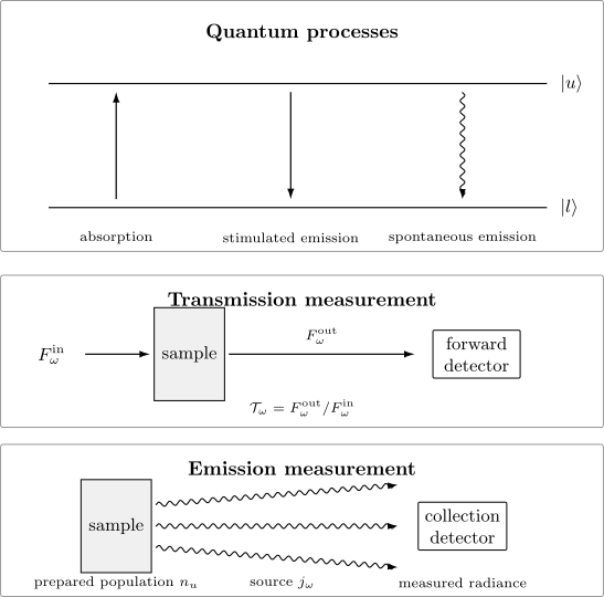
Absorption, stimulated emission, and spontaneous emission share the same level gap, but they enter experiments differently. Transmission compares an output beam with a reference input; emission measures radiance sourced by an upper-state population and filtered by collection optics.

Process ledger

The three processes can be kept straight with four questions:

• Absorption: the system starts in $l$; an incident resonant mode is required; the mode loses one photon; the rate scales with $n_l$ and field occupation.
• Stimulated emission: the system starts in $u$; an incident resonant mode is required; that mode gains one photon; the rate scales with $n_u$ and field occupation.
• Spontaneous emission: the system starts in $u$; no applied resonant field is required; one photon is emitted into an available mode; the free-space rate scales with $n_uA_{ul}$.
• Nonradiative relaxation: the system loses excitation without emitting the photon assigned to the observed branch; it changes populations and quantum yields but is neither absorption nor emission of that line.

Emission Spectra Versus Absorption Spectra

The same transition can have the same line center

For isolated stationary levels, both directions obey

$$\hbar\omega_{ul}=E_u-E_l.$$

An absorption line $l\rightarrow u$ and the reverse emission line $u\rightarrow l$ therefore share the same unperturbed transition frequency. Recoil, external fields, collisions, motion, and environment-dependent level shifts can modify the observed center, but there is no intrinsic rule that emission must occur at lower frequency for a two-level atom.

The initial populations are different

An integrated absorption feature is weighted primarily by the lower-state population,

$$\mathcal W_{lu}^{\mathrm{abs}} \propto n_l\Sigma_{lu}^{\mathrm{abs}},$$

with a stimulated-emission correction when $n_u$ is not negligible. An optically thin spontaneous-emission line is weighted by the upper-state population and branching rate,

$$\mathcal P_{ul}^{\mathrm{em}} \propto n_uA_{ul}\hbar\omega_{ul}.$$

Consequently, line-height or line-area ratios need not agree between the two spectra even when the same set of levels participates.

A spectrum is a network of branches

Suppose one upper level $u$ connects to several lower levels $l_1,l_2,\ldots$. Emission can display every radiative branch populated from $u$. Absorption from a cold sample may show only transitions originating in its ground level. Conversely, absorption can probe several populated lower levels that are not fed strongly by the prepared upper state in an emission experiment.

This network viewpoint is more reliable than trying to reflect one spectrum about a chosen frequency and call it the other.

Molecular relaxation and Stokes shifts

In a molecule or condensed environment, optical excitation can be followed by vibrational relaxation, solvent reorganization, internal conversion, or other nonradiative dynamics before emission. The emitting ensemble then starts from a different distribution than the absorbing ensemble. Emission often occurs at lower photon energy, producing a Stokes shift, but the shift is a dynamical and structural consequence rather than a definition of emission.

Approximate mirror-image relations between molecular absorption and emission bands require restrictive conditions: similar potential-energy curvatures, related vibrational wavefunctions, weak coordinate dependence of the electronic transition moment, and equilibrated sublevel populations. They fail under strong geometry changes, mode mixing, multiple conformers, non-Condon coupling, state-dependent broadening, or incomplete relaxation.

Profiles and spectral coordinates

Absorption and emission profiles can differ because they sample different inhomogeneous ensembles or relaxation histories. Even identical physical profiles look different after a nonlinear coordinate change. Since

$$\omega = \frac{2\pi c}{\lambda}, \qquad \left| \frac{d\omega}{d\lambda} \right| = \frac{2\pi c}{\lambda^2},$$

a density transforms as

$$X_\lambda(\lambda) = X_\omega(\omega) \frac{2\pi c}{\lambda^2}.$$

The area representing a conserved quantity is invariant only when the Jacobian is included. Peak positions and apparent symmetry on wavelength and frequency axes are not related by simply relabeling ticks.

Self-absorption and radiation trapping

Emission generated inside an optically thick sample can be reabsorbed before escaping. Photons near the strongest absorption frequency may undergo many absorption and re-emission events, lengthening the escape time and reshaping the observed line. In a spatially inhomogeneous source, cooler foreground material can carve an absorption reversal into an emission feature.

Thus the emergent spectrum can differ substantially from the local spontaneous emissivity. The correct object to propagate is radiance, not a bare Einstein coefficient.

Radiative Transfer

Source and extinction terms

Along one ray, neglecting frequency redistribution between different frequencies, the transfer equation is

$$\frac{dI_\omega}{ds} = -\alpha_\omega^{\mathrm{net}}I_\omega + j_\omega.$$

Stimulated emission is included as a negative contribution to $\alpha_\omega^{\mathrm{net}}$; spontaneous emission appears in the source term $j_\omega$. This bookkeeping avoids counting stimulated photons twice.

For a uniform slab with $\alpha_\omega^{\mathrm{net}}>0$, define

$$\tau_\omega = \alpha_\omega^{\mathrm{net}}L, \qquad S_\omega = \frac{j_\omega} {\alpha_\omega^{\mathrm{net}}}.$$

The formal solution is

$$I_\omega^{\mathrm{out}} = I_\omega^{\mathrm{in}} e^{-\tau_\omega} + S_\omega \left(1-e^{-\tau_\omega}\right).$$

The same material can therefore appear in absorption or emission relative to a background:

$$\begin{aligned} S_\omega<I_\omega^{\mathrm{in}} &\quad\Rightarrow\quad \text{a line depression}, \\ S_\omega>I_\omega^{\mathrm{in}} &\quad\Rightarrow\quad \text{a line enhancement}. \end{aligned}$$

“Absorption line” and “emission line” can consequently describe contrast against a background, not distinct microscopic transitions.

Local thermal equilibrium

In local thermodynamic equilibrium, microscopic detailed balance gives Kirchhoff’s relation

$$j_\omega = \alpha_\omega^{\mathrm{net}} B_\omega(T),$$

where the Planck spectral radiance per unit angular frequency is

$$B_\omega(T) = \frac{\hbar\omega^3} {4\pi^3c^2} \frac{1} {e^{\hbar\omega/(k_{\mathrm B}T)}-1}.$$

Thus $S_\omega=B_\omega(T)$ in LTE. An optically thick uniform source with no external background tends toward the Planck radiance. This statement links local emission and net absorption under equilibrium assumptions; it does not say that every laboratory fluorescence or discharge spectrum is a blackbody.

The historical and thermodynamic roles of the Planck spectrum belong to Planck’s Radiation Law.

Selection Rules and Intensities

Necessary conditions versus quantitative strengths

A symmetry selection rule tests whether a matrix element vanishes under a declared interaction. For electric-dipole transitions, parity and angular momentum severely constrain $d_{ul}^{(\epsilon)}$. The same conjugate matrix elements connect absorption and stimulated emission, and their mode sum also sets spontaneous emission.

An allowed transition is not guaranteed to be intense. Its measured signal also depends on:

• the magnitude of the nonzero matrix element;
• lower- or upper-state population;
• degeneracy averages and unresolved sums;
• polarization and observation direction;
• frequency factors, including the $\omega_{ul}^3$ scaling of a free-space electric-dipole $A$ coefficient;
• branching and nonradiative competition;
• line width, because area and peak height are different observables;
• optical depth and reabsorption; and
• collection and detector response.

Likewise, “forbidden” means that a specified leading matrix element vanishes in an idealized symmetry limit. Magnetic-dipole, electric-quadrupole, two-photon, collision-induced, or mixing-enabled channels can still produce observable lines.

Polarization-resolved spectra

If magnetic sublevels are resolved, the spherical polarization component $q=0,\pm1$ selects changes in magnetic quantum number. Absorption prepares an anisotropic excited-state distribution when the pump is polarized. Subsequent emission then carries angular and polarization information about that distribution.

Summing over polarizations or averaging over initial sublevels can erase this information. A database strength quoted for an unresolved level-to-level transition must not be inserted into a polarization-resolved calculation without unpacking its averaging convention.

From intrinsic strength to a measured line

A useful factorization for an optically thin emission count rate is

$$\dot N_{ul}^{\mathrm{det}} = N_u A_{ul} \eta_{ul}^{\mathrm{prop}} \eta_{ul}^{\mathrm{coll}} \eta_{ul}^{\mathrm{det}},$$

where $N_u$ is the number of emitters in the viewed volume and the three $\eta$ factors represent escape or propagation, collection, and detector efficiency. For spectral counts, multiply by the normalized emitted profile and convolve with the instrument response.

For weak absorption, a corresponding detected photon deficit is

$$\Delta\dot N_\omega^{\mathrm{det}} \simeq \dot N_{\omega,\mathrm{in}} \tau_\omega \eta_\omega^{\mathrm{det}},$$

only when $\tau_\omega\ll1$ and additive backgrounds are negligible. These relations show why observed intensity is not a synonym for transition probability.

Temperature Effects

Thermal populations

For a system in internal thermal equilibrium,

$$\begin{aligned} n_i(T) &= n \frac{g_i e^{-E_i/(k_{\mathrm B}T)}} {Z(T)}, \\ Z(T) &= \sum_j g_j e^{-E_j/(k_{\mathrm B}T)}. \end{aligned}$$

Absorption is weighted by lower-state populations. Raising temperature can deplete a ground-state line, populate rotational or vibrational hot bands, and redistribute intensity over many transitions. Spontaneous emission is weighted by whatever upper-state distribution the preparation and relaxation actually create; that distribution need not be thermal.

Stimulated-emission correction in equilibrium

In LTE,

$$\frac{n_u}{n_l} = \frac{g_u}{g_l} e^{-\hbar\omega_{ul}/(k_{\mathrm B}T)}.$$

Combining this ratio with the degeneracy-weighted stimulated cross section gives

$$\alpha_\omega^{\mathrm{net}} = n_l \sigma_{lu}^{\mathrm{abs}}(\omega) \left[ 1-e^{-\hbar\omega_{ul}/(k_{\mathrm B}T)} \right].$$

At optical frequencies and ordinary temperatures, the exponential is often negligible and true absorption dominates. At microwave or far-infrared frequencies, stimulated emission can substantially reduce net attenuation. Omitting this factor biases line intensities and inferred column densities.

Temperature changes more than populations

Temperature can also change:

• Doppler widths through the velocity distribution;
• collisional widths and shifts through collision rates;
• molecular partition functions and isotopologue populations;
• chemical composition or ionization balance;
• nonradiative quenching rates; and
• the ambient thermal photon occupation.

One should therefore state what temperature a spectral fit measures. A rotational temperature, vibrational temperature, electronic excitation temperature, translational temperature, and radiation temperature coincide only in genuine equilibrium.

Excitation temperature and inversion

For any pair of levels with positive populations, define an excitation temperature by

$$\frac{n_u}{n_l} = \frac{g_u}{g_l} \exp\!\left[ -\frac{\hbar\omega_{ul}} {k_{\mathrm B}T_{\mathrm{ex}}} \right].$$

This is a parametrization, not proof of thermal equilibrium. If $n_u/g_u>n_l/g_l$, then $T_{\mathrm{ex}}<0$ for the two-level ratio and the line has small-signal gain. Other degrees of freedom can still have positive temperatures.

Worked Example: One Upper Level, Two Lower Levels

Consider nondegenerate levels

$$\begin{aligned} E_0&=0, \\ E_1&=0.10\ \mathrm{eV}, \\ E_u&=2.50\ \mathrm{eV}. \end{aligned}$$

At $T=300\ \mathrm K$, suppose the two lower levels are thermalized. Their population ratio is

$$\frac{n_1}{n_0} = \exp\!\left( -\frac{0.10\ \mathrm{eV}} {k_{\mathrm B}(300\ \mathrm K)} \right) \simeq 2.1\times10^{-2}.$$

Now prepare level $u$ by some independent pump and let

$$\begin{aligned} A_{u0}&=6.0\times10^7\ \mathrm{s}^{-1}, \\ A_{u1}&=2.0\times10^7\ \mathrm{s}^{-1}. \end{aligned}$$

For nondegenerate electric-dipole lines, the reciprocal strength relations give

$$\Sigma_{lu}^{\mathrm{abs}} \propto f_{lu} \propto \frac{A_{ul}}{\omega_{ul}^2}.$$

The ratio of integrated absorption cross sections is therefore

$$\begin{aligned} \frac{\Sigma_{1u}^{\mathrm{abs}}} {\Sigma_{0u}^{\mathrm{abs}}} &= \frac{A_{u1}}{A_{u0}} \left( \frac{\omega_{u0}}{\omega_{u1}} \right)^2 \\ &= \frac{1}{3} \left(\frac{2.50}{2.40}\right)^2 \simeq 0.362. \end{aligned}$$

Hence the hot-band absorption area at photon energy $2.40\ \mathrm{eV}$ is

$$\frac{\mathcal W_{1u}^{\mathrm{abs}}} {\mathcal W_{0u}^{\mathrm{abs}}} = \frac{n_1}{n_0} \frac{\Sigma_{1u}^{\mathrm{abs}}} {\Sigma_{0u}^{\mathrm{abs}}} \simeq 7.6\times10^{-3}.$$

It is only about $0.76\%$ of the ground-state absorption area at $2.50\ \mathrm{eV}$.

The radiative branching fractions are

$$b_{u0}=0.75, \qquad b_{u1}=0.25.$$

For equal collection efficiency and optically thin propagation, the emitted power ratio is

$$\begin{aligned} \frac{P_{u0}}{P_{u1}} &= \frac{A_{u0}\omega_{u0}} {A_{u1}\omega_{u1}} \\ &= 3\left(\frac{2.50}{2.40}\right) \simeq 3.13. \end{aligned}$$

The weaker emission line therefore carries about $32\%$ of the power of the stronger line, even though absorption from its lower state was only about $0.76\%$ as strong. The transition network is the same; the initial populations are not.

Practical Interpretation Workflow

1. Name the measured quantity. Distinguish transmittance, absorbance, optical depth, photon counts, power, radiance, and a fitted line area.
2. Declare the spectral coordinate. Record whether the density is per frequency, angular frequency, wavenumber, wavelength, or energy.
3. Identify initial populations. Absorption starts in lower states; emission starts in upper states. State whether populations are thermal, pumped, state selected, or inferred.
4. Specify the interaction and polarization. Do not apply an electric- dipole rule to a magnetic-dipole or Raman observable.
5. Separate strength from shape. Compare integrated areas when testing intrinsic strengths; compare widths and profiles only with a broadening model.
6. Estimate optical depth. Decide whether Beer–Lambert attenuation, optically thin emission, or full radiative transfer is appropriate.
7. Account for branching and quenching. A short observed lifetime or weak emission need not imply a small absorption matrix element.
8. Propagate through the instrument. Include finite resolution, collection solid angle, throughput, detector response, and backgrounds.
9. Attach uncertainties and provenance. Database values may be observed, calculated, fitted, or critically evaluated, with different conventions.

Common Mistakes

Treating an absorption dip as an excited-state probability

The fractional beam loss is a propagation observable. It depends on column density, optical depth, scattering, backgrounds, and collection geometry. It is not generally the Born probability that one selected system is excited.

Calling every decrease in transmission absorption

Elastic scattering, reflection, beam steering, and detector nonlinearities can all lower the forward signal. Control measurements are part of the physical definition of the observable.

Equating spontaneous and stimulated emission

Both end in the lower state, but spontaneous emission supplies a source term across available modes, whereas stimulated emission modifies propagation in an occupied mode.

Assuming absorption and emission spectra are mirror images

The spectra start from different populations and can follow different relaxation pathways. Mirror-image behavior is an approximation for restricted molecular cases, not a general reciprocity theorem.

Ignoring stimulated emission in thermal absorption

At low photon energy relative to $k_{\mathrm B}T$, upward and downward stimulated events nearly cancel. The net coefficient contains $1-e^{-\hbar\omega/(k_{\mathrm B}T)}$.

Comparing peak heights as transition strengths

Peak height depends on width, profile, resolution, and saturation. Integrated area is often closer to the intrinsic strength, provided overlap and continuum subtraction are controlled.

Mixing photon spectra and power spectra

A power spectrum weights each detected photon by $\hbar\omega$. Detector counts and radiated energy therefore have different line ratios unless the frequencies are effectively equal.

Forgetting the spectral Jacobian

A density per wavelength is not obtained from a density per frequency by changing only the axis label. The Jacobian changes both profile shape and peak location.

Applying Beer–Lambert through an emitting sample

When $j_\omega$ is appreciable, transmission is not a pure exponential of absorption. The source term can fill the line or turn it into net emission.

Inferring equilibrium from one Boltzmann-looking ratio

An excitation temperature describes one population ratio. Different level pairs can yield different temperatures in a non-LTE source.

Key Takeaways

1. Absorption, stimulated emission, and spontaneous emission connect the same level gap but enter spectra through different initial populations and field conditions.
2. Weak absorption is naturally described by cross section, column density, and optical depth; optically thin emission is described by upper-state population, $A$ coefficient, and collection geometry.
3. Stimulated emission subtracts from net extinction and produces gain when population per sublevel is larger upstairs than downstairs.
4. Absorption and emission spectra need not share line ratios, envelopes, or apparent shapes even when they involve the same states.
5. The transfer equation unifies absorption and emission: contrast depends on both optical depth and the source function relative to the background.
6. Temperature changes populations, stimulated-emission corrections, broadening, and sometimes chemistry; a fitted spectral temperature must be named precisely.
7. Measured intensity is a product of intrinsic strength, populations, propagation, branching, and instrument response.

Exercises

Exercise 1: Infer a cross section from transmission

A dilute sample has lower-state column density $\mathcal N_l=2.0\times10^{16}\ \mathrm{m}^{-2}$. At line center, the measured transmittance is $\mathcal T=0.370$. Assume pure Beer–Lambert absorption. Find the line-center cross section and the base-ten absorbance.

Solution

The optical depth is

$$\tau = -\ln(0.370) = 0.994.$$

Therefore

$$\sigma = \frac{\tau}{\mathcal N_l} = 4.97\times10^{-17}\ \mathrm{m}^2.$$

The base-ten absorbance is

$$\mathcal A_{10} = -\log_{10}(0.370) = 0.432,$$

which also equals $\tau/\ln 10$.

Exercise 2: Photon counts versus emitted power

Two optically thin emission lines produce equal photon rates. Their angular frequencies are $\omega$ and $2\omega$. Compare their photon-count ratio and their radiated-power ratio, assuming equal detector efficiencies.

Solution

The photon-count ratio is one by assumption. Each photon carries energy $\hbar\omega$, so

$$\frac{P_{2\omega}}{P_{\omega}} = \frac{\hbar(2\omega)} {\hbar\omega} =2.$$

Equal photon spectra are not equal power spectra.

Exercise 3: Thermal stimulated-emission correction

Evaluate the LTE correction

$$C(x)=1-e^{-x}, \qquad x=\frac{\hbar\omega}{k_{\mathrm B}T},$$

for $x=0.25$ and $x=10$. Interpret the result.

Solution

For $x=0.25$,

$$C(0.25) = 1-e^{-0.25} \simeq 0.221.$$

Net attenuation is only about $22.1\%$ of the lower-population absorption term; thermal stimulated emission cancels the remaining $77.9\%$.

For $x=10$,

$$C(10) = 1-e^{-10} \simeq 0.999955.$$

Stimulated emission is negligible in the second case. This is the usual optical-frequency regime at modest temperature.

Exercise 4: Absorption and emission line ratios

An upper level $u$ radiates to two nondegenerate lower levels $a$ and $b$. The photon energies are $2.0\ \mathrm{eV}$ and $1.0\ \mathrm{eV}$, while

$$\begin{aligned} A_{ua}&=4.0\times10^7\ \mathrm{s}^{-1}, \\ A_{ub}&=1.0\times10^7\ \mathrm{s}^{-1}. \end{aligned}$$

The lower-state populations satisfy $n_b/n_a=0.10$, and the two integrated absorption cross sections are equal. The quoted $A$ values are consistent with the nondegenerate electric-dipole relation $A\propto\omega^2f$. Find the absorption-area ratio $\mathcal W_{bu}/\mathcal W_{au}$, the emitted photon-rate ratio $\dot N_{ua}/\dot N_{ub}$, and the emitted-power ratio $P_{ua}/P_{ub}$.

Solution

Equal integrated cross sections give

$$\frac{\mathcal W_{bu}} {\mathcal W_{au}} = \frac{n_b}{n_a} =0.10.$$

The optically thin photon-rate ratio is the ratio of $A$ coefficients:

$$\frac{\dot N_{ua}} {\dot N_{ub}} = \frac{A_{ua}}{A_{ub}} =4.0.$$

Power includes photon energy:

$$\frac{P_{ua}}{P_{ub}} = \frac{A_{ua}(2.0\ \mathrm{eV})} {A_{ub}(1.0\ \mathrm{eV})} = 8.0.$$

The same transition network produces very different absorption and emission ratios because the initial-state weights differ.

Exercise 5: Solve a uniform transfer slab

Starting from

$$\frac{dI_\omega}{ds} = -\alpha_\omega I_\omega+j_\omega,$$

derive the emergent radiance of a uniform slab. Then take $\tau_\omega=1$ and evaluate $I_\omega^{\mathrm{out}}/S_\omega$ for $I_\omega^{\mathrm{in}}=5S_\omega$ and for $I_\omega^{\mathrm{in}}=0$.

Solution

For constant coefficients, multiply by $e^{\alpha_\omega s}$ and integrate. With $S_\omega=j_\omega/\alpha_\omega$ and $\tau_\omega=\alpha_\omega L$,

$$I_\omega^{\mathrm{out}} = I_\omega^{\mathrm{in}}e^{-\tau_\omega} + S_\omega(1-e^{-\tau_\omega}).$$

For $I_\omega^{\mathrm{in}}=5S_\omega$ and $\tau_\omega=1$,

$$\frac{I_\omega^{\mathrm{out}}}{S_\omega} = 5e^{-1}+1-e^{-1} = 1+\frac{4}{e} \simeq 2.47.$$

The slab makes a depression relative to the background value $5S_\omega$. With no incident background,

$$\frac{I_\omega^{\mathrm{out}}}{S_\omega} = 1-e^{-1} \simeq 0.632,$$

so the same slab appears in emission.

Exercise 6: A two-line temperature diagnostic

Two optically thin lines originate from thermalized upper levels $u_1$ and $u_2$ of the same species. Let

$$E_{u_2}-E_{u_1}=0.12\ \mathrm{eV},$$

and suppose

$$\frac{g_{u_2}A_2\omega_2} {g_{u_1}A_1\omega_1} =2.0.$$

The measured power ratio is $P_2/P_1=0.50$. Neglect optical-depth and detector-response differences. Find the excitation temperature.

Solution

Thermal upper-state populations give

$$\frac{P_2}{P_1} = 2.0 \exp\!\left[ -\frac{0.12\ \mathrm{eV}} {k_{\mathrm B}T} \right].$$

Thus the exponential equals $0.25$, and

$$T = \frac{0.12\ \mathrm{eV}} k_{\mathrm B}\ln 4 \simeq 1.00\times10^3\ \mathrm K.$$

The result is an excitation temperature for the assumed level population model. It equals the kinetic temperature only if the source is thermalized.

Exercise 7: Transform a normalized spectrum

Let $\phi_\omega(\omega)$ be normalized in angular frequency. Derive the corresponding wavelength profile $\phi_\lambda(\lambda)$ and verify its normalization. Why can a symmetric frequency profile be asymmetric in wavelength?

Solution

Conservation of probability or spectral weight requires

$$\phi_\lambda(\lambda)\,d\lambda = \phi_\omega(\omega)\,|d\omega|.$$

Since $\omega=2\pi c/\lambda$,

$$\phi_\lambda(\lambda) = \phi_\omega\!\left(\frac{2\pi c}{\lambda}\right) \frac{2\pi c}{\lambda^2}.$$

Changing variables back to $\omega$ gives

$$\int_0^\infty \phi_\lambda(\lambda)\,d\lambda = \int_0^\infty \phi_\omega(\omega)\,d\omega =1.$$

The nonlinear map $\lambda=2\pi c/\omega$ and its $1/\lambda^2$ Jacobian distort symmetry and shift the plotted maximum.

Exercise 8: Test for population inversion

A transition has $g_l=2$, $g_u=6$, and $n_u/n_l=4$. Assume matched absorption and stimulated-emission profiles. Determine whether the line has small-signal absorption or gain, and express $\alpha_\omega^{\mathrm{net}}$ in units of $n_l\sigma_{lu}^{\mathrm{abs}}(\omega)$.

Solution

The degeneracy relation gives

$$\sigma_{ul}^{\mathrm{st}} = \frac{g_l}{g_u} \sigma_{lu}^{\mathrm{abs}} = \frac{1}{3} \sigma_{lu}^{\mathrm{abs}}.$$

Hence

$$\begin{aligned} \frac{\alpha_\omega^{\mathrm{net}}} {n_l\sigma_{lu}^{\mathrm{abs}}} &= 1- \frac{n_u}{n_l} \frac{g_l}{g_u} \\ &= 1-\frac{4}{3} = -\frac{1}{3}. \end{aligned}$$

The coefficient is negative, so the weak probe is amplified. Equivalently, $n_u/g_u>n_l/g_l$.

Cross-Links

• Spectroscopy Nomenclature separates transmittance, decadic and Napierian absorbance, absorptance, optical depth, and absorption versus extinction cross sections.
• Einstein Coefficient Reference gives convention-labeled $A/B$ relations and separates intrinsic coefficients from field- and population-dependent signals.
• Oscillator Strength Reference gives the integrated-area formulas and spectral-coordinate Jacobians for E1 absorption.
• Line Shape Reference supplies normalized Lorentzian, Gaussian, and Voigt profiles for cross-section and optical-depth models.
• Spectroscopy
• Transition Rates
• Oscillator Strengths
• Einstein Coefficients
• Line Shapes and Broadening
• Electronic Spectroscopy
• Fluorescence and Phosphorescence
• Infrared Spectroscopy
• Atomic Selection Rules
• Dipole Transitions
• Transition Rates in Light–Matter Interaction
• Optical Bloch Equations
• Planck’s Radiation Law
• Spectroscopy as an Experimental Technique

References

• R. C. Hilborn, “Einstein coefficients, cross sections, $f$ values, dipole moments, and all that,” American Journal of Physics 50, 982-986 (1982), doi:10.1119/1.12937; revised version, arXiv:physics/0202029.
• C. Cohen-Tannoudji, J. Dupont-Roc, and G. Grynberg, Atom–Photon Interactions: Basic Processes and Applications, Wiley, 1992.
• R. Loudon, The Quantum Theory of Light, 3rd ed., Oxford University Press, 2000.
• C. J. Foot, Atomic Physics, Oxford University Press, 2005.
• P. F. Bernath, Spectra of Atoms and Molecules, 5th ed., Oxford University Press, 2025, doi:10.1093/oso/9780197754498.001.0001.
• W. Demtröder, Laser Spectroscopy 1: Basic Principles, 5th ed., Springer, 2014, doi:10.1007/978-3-642-53859-9.
• G. B. Rybicki and A. P. Lightman, Radiative Processes in Astrophysics, Wiley, 1979.
• A. Kramida, “Spectral Lines: Selection Rules, Intensities, Transition Probabilities, Values, and Line Strengths,” in Atomic Spectroscopy: An Introduction, National Institute of Standards and Technology, accessed 2026-07-22.
• NIST, Atomic Spectra Database: Spectral Lines Help, including definitions of observed intensities, transition probabilities, oscillator strengths, and line strengths, accessed 2026-07-22.
• HITRAN, Definitions and Units, including line intensity, lower-state energy, temperature scaling, absorption coefficient, and optical depth conventions, accessed 2026-07-22.
• IUPAC, “Quantum yield”, Compendium of Chemical Terminology, 5th ed., online version 5.0.0, 2025, doi:10.1351/goldbook.Q04991.