Oscillator Strengths

An oscillator strength is a dimensionless, energy-weighted measure of an electric-dipole transition. For absorption from a nondegenerate state $|i\rangle$ to a higher state $|f\rangle$, the standard isotropic definition in SI units is

$$\begin{gathered} f_{if} = \frac{2m_e\omega_{fi}} {3\hbar e^2} \left| \langle f|\widehat{\mathbf D}|i\rangle \right|^2, \\ \omega_{fi} = \frac{E_f-E_i}{\hbar}>0. \end{gathered}$$

Here $\widehat{\mathbf D}$ is the electric-dipole operator, $m_e$ is the electron mass, and $e>0$ is the elementary charge. The factor multiplying the matrix element normalizes the quantum transition to the response of a classical electron oscillator. It does not make $f_{if}$ a probability: an oscillator strength has no observation time, is not restricted to the interval $[0,1]$, and by itself is neither a rate nor a peak cross section.

Oscillator strengths are valuable because they connect several descriptions of the same electric-dipole line:

• a transition dipole or reduced line strength from structure theory;
• an integrated absorption cross section;
• an Einstein $A$ coefficient after frequency and degeneracy factors are supplied;
• exact and approximate sum rules over complete sets of final states.

Those connections are convention-sensitive. A quoted value is incomplete unless the states, degeneracy average, polarization average, transition energy, and line grouping are known.

Canonical Scope

This page owns the definition and interpretation of electric-dipole oscillator strengths in atomic and molecular spectroscopy. It develops the state-to-state and level-averaged conventions, explains the Thomas–Reiche–Kuhn sum rule as a strength budget, and relates $f$ values to frequency-integrated absorption.

Neighboring pages retain distinct canonical roles:

• Transition Rates owns the general workflow from perturbative amplitudes to channel rates and recorded signals.
• Sum Rules and Completeness Tricks owns the commutator derivation of energy-weighted quantum sum rules.
• Transition Rates in Light–Matter Interaction owns quantized-field absorption and emission rates.
• Multi-Electron Atoms owns configuration mixing, term structure, and reduced atomic line strengths.
• Electronic Structure Overview owns the broader electronic-state calculation problem for molecules.
• Many-Body Sum Rules owns response-function moments and many-body spectral-weight constraints.

The formulas below therefore emphasize spectroscopic conversion and bookkeeping rather than duplicating those derivations.

Convention Ledger

Throughout the main development:

• $i$ labels the lower state or level and $f$ the upper state or level;
• $f_{if}>0$ denotes an absorption oscillator strength;
• $\omega_{fi}=(E_f-E_i)/\hbar>0$;
• $g_i$ and $g_f$ denote initial- and final-level statistical weights;
• $L_\nu$ and $L_\omega$ are line profiles normalized to unit area in their stated spectral coordinates;
• vacuum SI electromagnetic conventions are used unless atomic units are explicitly declared;
• oscillator strength without a multipole label means electric dipole, E1.

The same symbol $f$ is used in the literature for state-to-state, level-to-level, multiplet, band, and signed reverse-transition quantities. The IUPAC Gold Book explicitly warns that differing uses exist. Subscripts alone do not resolve the ambiguity.

Dipole Matrix Elements

Interaction with an electric field

In the long-wavelength electric-dipole approximation, the interaction with a classical field is

$$\widehat V(t) = -\widehat{\mathbf D} \mathbin{\cdot} \mathbf E(t).$$

For $N$ electrons with positions measured from a fixed origin,

$$\widehat{\mathbf D}_{\mathrm{el}} = -e\sum_{a=1}^{N}\widehat{\mathbf r}_a.$$

For a molecule, the full dipole operator also contains the nuclear charges:

$$\widehat{\mathbf D} = e\sum_A Z_A\widehat{\mathbf R}_A -e\sum_{a=1}^{N}\widehat{\mathbf r}_a.$$

The transition dipole is

$$\mathbf D_{fi} = \langle f| \widehat{\mathbf D} |i\rangle.$$

For two orthogonal exact states of a fixed-charge system, translating the coordinate origin adds a constant multiple of $\langle f|i\rangle$ and therefore does not change the transition dipole. Permanent dipoles of charged systems require more care because the corresponding diagonal overlap is one.

The transition matrix element contains the structure physics. Symmetry can make it vanish, configuration mixing can redistribute it, and vibronic or spin–orbit coupling can lend intensity to a transition that is forbidden in a simpler model.

Polarization-resolved coupling

For a unit polarization vector $\boldsymbol{\epsilon}$, the field probes

$$D_{fi}^{(\epsilon)} = \boldsymbol{\epsilon} \mathbin{\cdot} \mathbf D_{fi}.$$

The corresponding directional oscillator strength is

$$f_{if}^{(\epsilon)} = \frac{2m_e\omega_{fi}} {\hbar e^2} \left| \boldsymbol{\epsilon} \mathbin{\cdot} \mathbf D_{fi} \right|^2.$$

For an isotropic ensemble or an average over three mutually orthogonal polarizations,

$$\begin{aligned} \overline{ \left| \boldsymbol{\epsilon} \mathbin{\cdot} \mathbf D_{fi} \right|^2 } &= \frac{1}{3} \left| \mathbf D_{fi} \right|^2, \\ f_{if} &= \frac{1}{3} \sum_{\alpha=x,y,z} f_{if}^{(\alpha)}. \end{aligned}$$

The factor $1/3$ is an orientation or polarization average, not a dynamical suppression. It must not be inserted again when a tabulated quantity is already isotropically averaged.

For oriented molecules, aligned samples, Zeeman-resolved atoms, or polarization-selective detection, the component strengths are the physically relevant quantities. An isotropic $f$ value then discards information needed to predict the experiment.

Line strength and reduced matrix elements

A line strength is the squared transition matrix element before the transition-energy factor is applied. For an atomic E1 transition between angular-momentum levels,

$$S_{if} = \left| \left\langle \gamma_fJ_f \left\| \widehat D^{(1)} \right\| \gamma_iJ_i \right\rangle \right|^2.$$

Here $\gamma_i$ and $\gamma_f$ collect all other labels. With the usual reduced-matrix-element convention and an unpolarized initial level,

$$f_{if} = \frac{2m_e\omega_{fi}} {3\hbar e^2g_i} S_{if}, \qquad g_i=2J_i+1.$$

The factor $1/g_i$ averages over initial magnetic substates. The reduced line strength already represents the appropriate sums over magnetic substates and spherical components. Adding an extra magnetic-substate sum to this formula double counts degeneracy.

For hyperfine-resolved data, $g_i=2F_i+1$ if the stated line connects definite $F$ levels. For term-to-term or multiplet strengths, the adopted line grouping and statistical weights must be stated separately.

Length and velocity forms

For a nonrelativistic Hamiltonian with canonical kinetic energy and local coordinate-dependent potentials, define

$$\widehat{\mathbf R} = \sum_{a=1}^{N}\widehat{\mathbf r}_a, \qquad \widehat{\mathbf P} = \sum_{a=1}^{N}\widehat{\mathbf p}_a.$$

The commutator relation

$$\left[ \widehat H, \widehat{\mathbf R} \right] = -\frac{i\hbar}{m_e} \widehat{\mathbf P}$$

gives, between exact eigenstates,

$$\langle f|\widehat{\mathbf P}|i\rangle = \frac{im_e(E_f-E_i)}{\hbar} \langle f|\widehat{\mathbf R}|i\rangle.$$

Consequently the length and velocity forms agree:

$$\begin{aligned} f_{if}^{(L)} &= \frac{2m_e(E_f-E_i)} {3\hbar^2} \left| \langle f|\widehat{\mathbf R}|i\rangle \right|^2, \\ f_{if}^{(V)} &= \frac{2} {3m_e(E_f-E_i)} \left| \langle f|\widehat{\mathbf P}|i\rangle \right|^2. \end{aligned}$$

These equations are written for nondegenerate states. Initial-state averages or reduced-matrix-element conventions add the corresponding degeneracy factors.

Approximate wavefunctions generally give different length- and velocity-form values. Their disagreement is a useful convergence diagnostic, but it is not automatically a statistical uncertainty. Nonlocal pseudopotentials, relativistic Hamiltonians, incomplete response terms, and inconsistent operators can modify the simple commutator relation, so apparent agreement is not by itself proof of accuracy.

Oscillator Strength Definition

State-to-state absorption strength

Using

$$\widehat{\mathbf D}_{\mathrm{el}} = -e\widehat{\mathbf R},$$

the isotropic state-to-state definition can be written in either dipole or coordinate form:

$$\begin{aligned} f_{if} &= \frac{2m_e\omega_{fi}} {3\hbar e^2} \left| \mathbf D_{fi} \right|^2 \\ &= \frac{2m_e(E_f-E_i)} {3\hbar^2} \left| \langle f|\widehat{\mathbf R}|i\rangle \right|^2. \end{aligned}$$

The sign of the electronic charge disappears after taking the modulus squared. The energy factor remains essential: two transitions with the same dipole matrix element but different frequencies do not have the same oscillator strength.

Dimensional analysis provides a quick check:

$$\frac{m_e\omega}{\hbar e^2} \left| \mathbf D \right|^2 \sim \frac{\mathrm{kg}\,\mathrm{s}^{-1}} {\mathrm{J\,s}\,\mathrm{C}^2} \left(\mathrm{C\,m}\right)^2 =1.$$

Atomic-unit form

In atomic units,

$$m_e=e=\hbar=1.$$

For a level-to-level E1 transition whose reduced line strength is in $e^2a_0^2$ and whose energy separation is in hartrees,

$$f_{if} = \frac{2}{3} \frac{\Delta E}{g_i} S_{if}, \qquad \Delta E=E_f-E_i.$$

For nondegenerate states, set $g_i=1$ and interpret $S$ as the squared vector transition dipole in atomic units. A common error is to insert an energy in electronvolts into this atomic-unit formula.

Reverse transitions and signed strengths

The absorption oscillator strength $f_{if}$ is normally quoted as a positive number for $E_f>E_i$. If the same algebraic definition is extended to the reverse transition without replacing the energy difference by its absolute value, then

$$f_{fi}<0.$$

For level-averaged strengths,

$$g_i f_{if} = -g_f f_{fi}.$$

The negative sign is useful in sum rules because downward transitions from an excited initial state contribute negative spectral weight. It does not mean that an emission probability or rate is negative. Databases commonly list positive absorption $f$ values even when the corresponding $A$ coefficient describes downward emission.

The f, gf, log(gf), S, and A ledger

Several quantities that appear side by side in line lists are related but not interchangeable:

• $f_{if}$ is dimensionless and usually averages over the lower level’s substates.
• $g_if_{if}$ removes that lower-level average and is abbreviated $gf$.
• $\log(gf)$ means $\log_{10}(g_if_{if})$ in standard atomic line lists.
• $S_{if}$ is a squared matrix element and carries dipole-squared units unless atomic units are declared.
• $A_{fi}$ is a spontaneous-emission rate in inverse seconds and averages over the upper level’s substates.

For an E1 line in vacuum,

$$\begin{aligned} A_{fi} &= \frac{e^2\omega_{fi}^{\,2}} {2\pi\epsilon_0m_ec^3} \frac{g_i}{g_f} f_{if} \\ &= \frac{\omega_{fi}^{\,3}} {3\pi\epsilon_0\hbar c^3g_f} S_{if}. \end{aligned}$$

Equivalently, with vacuum wavelength $\lambda=2\pi c/\omega_{fi}$,

$$A_{fi} = \frac{2\pi e^2} {m_ec\epsilon_0\lambda^2} \frac{g_i}{g_f} f_{if}.$$

These conversions assume the same E1 line, the same level grouping, and consistent degeneracy conventions. They do not apply unchanged in a dielectric medium. Magnetic-dipole, electric-quadrupole, and higher-multipole transitions have their own line strengths and rate formulas; NIST generally does not assign oscillator strengths to those forbidden-transition multipoles.

Einstein Coefficients owns the detailed-balance derivation of the $A$ and $B$ relations, their spectral-energy-density conventions, and their blackbody connection.

Why an oscillator strength can exceed one

An individual $f$ value is not a Bernoulli probability. In a many-electron system, collective or strongly allowed transitions can carry oscillator strength larger than one. What is constrained under the assumptions of the Thomas–Reiche–Kuhn rule is the complete signed sum, not each term separately.

Even for a one-electron system, excited-state upward strengths can exceed one because negative downward contributions must also be included in the signed sum.

Sum Rules

The Thomas–Reiche–Kuhn budget

For $N$ nonrelativistic electrons governed by a Hamiltonian with local coordinate-dependent interactions, the isotropic oscillator strengths from a fixed exact state obey

$$\sum_f f_{if}=N.$$

The symbol $\sum_f$ is shorthand for a complete spectral resolution:

$$\begin{aligned} \sum_f &\longrightarrow \sum_{f\in\mathrm{bound}} \\ &\quad+ \sum_{\mathrm{channels}} \int_{\mathrm{continuum}} dE\,\rho_f(E). \end{aligned}$$

The continuum density and continuum-state normalization must be used consistently. A list of discrete bound lines generally does not exhaust the rule.

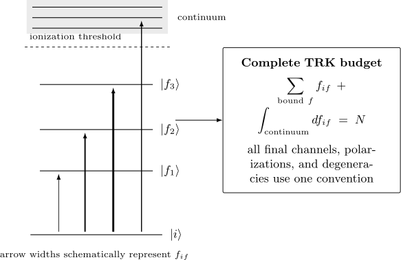
Schematic distribution of oscillator strength among bound lines and a continuum. Arrow widths represent relative strengths only. The exact Thomas–Reiche–Kuhn sum requires a complete set of final channels and a single polarization, degeneracy, and sign convention.

For one Cartesian component,

$$\sum_f \frac{2m_e(E_f-E_i)} {\hbar^2} \left| \langle f|\widehat R_\alpha|i\rangle \right|^2 =N.$$

Averaging the three Cartesian component rules gives the isotropic form. The underlying identity is

$$\begin{aligned} &\sum_f (E_f-E_i) \langle i|\widehat R_\alpha|f\rangle \langle f|\widehat R_\beta|i\rangle \\ &\qquad= \frac{1}{2} \langle i| \left[ \widehat R_\alpha, \left[ \widehat H,\widehat R_\beta \right] \right] |i\rangle. \end{aligned}$$

For the stated Hamiltonian, the double commutator is

$$\left[ \widehat R_\alpha, \left[ \widehat H,\widehat R_\beta \right] \right] = \frac{N\hbar^2}{m_e} \delta_{\alpha\beta}.$$

The full derivation and the general completeness method are given in Sum Rules and Completeness Tricks.

Conditions and qualifications

The simple right-hand side $N$ assumes:

• nonrelativistic canonical electron kinetic energy;
• a consistent electric-dipole operator;
• local coordinate-dependent potentials;
• exact eigenstates of the same Hamiltonian;
• a complete discrete-plus-continuum final-state set;
• signed energy differences for an excited initial state;
• all required polarizations and unresolved degeneracies treated according to one convention.

Relativistic corrections, nonlocal effective potentials, projected few-level models, and energy-dependent effective Hamiltonians can change the commutator or move strength outside the modeled space. A failed partial sum does not identify which assumption is responsible.

For an excited initial state, the signed rule is

$$\begin{aligned} \sum_{E_f>E_i}f_{if} + \sum_{E_f<E_i}f_{if} &=N, \\ f_{if}<0 &\quad(E_f<E_i). \end{aligned}$$

Summing only positive upward strengths from an excited state need not yield $N$ and can exceed it.

Harmonic-oscillator saturation

The one-dimensional harmonic oscillator gives a transparent example. For a single electron,

$$\widehat x = \sqrt{\frac{\hbar}{2m_e\Omega}} \left( \widehat a+\widehat a^\dagger \right).$$

From the ground state, only $|1\rangle$ has a nonzero dipole matrix element:

$$\left| \langle 1|\widehat x|0\rangle \right|^2 = \frac{\hbar}{2m_e\Omega}.$$

The directional oscillator strength is therefore

$$f_{01}^{(x)} = \frac{2m_e\Omega}{\hbar} \frac{\hbar}{2m_e\Omega} =1.$$

One line saturates the one-electron, one-component sum rule. Real atoms and molecules distribute the same kind of budget across many bound, continuum, electronic, vibronic, and rotational channels.

Partial sums as diagnostics

Define a cumulative sum through an energy cutoff:

$$F_i(E_{\max}) = \sum_{E_f\le E_{\max}}f_{if}.$$

For a ground state, $F_i$ is nondecreasing when all included channels are ordinary upward E1 transitions. It approaches $N$ only after the continuum and sufficiently high-energy states are included. Its behavior can diagnose:

• missing diffuse or continuum basis functions;
• omitted symmetry or ionization channels;
• inconsistent degeneracy factors;
• accidental mixing of length- and velocity-form data;
• double-counted multiplet components;
• a truncated active-electron model whose effective sum is not the physical electron count.

Agreement with the final sum is necessary but not sufficient for accurate individual lines. Large positive and negative errors can cancel, and a basis can reproduce a global moment while misplacing strength spectrally.

Relation to many-body response

The oscillator-strength rule is an energy-weighted moment of a dipole response. In extended or interacting systems, analogous constraints appear as $f$-sum rules for density and current response. Collective modes can carry substantial spectral weight while the exact total remains fixed by commutators and conservation laws. The response-function formulation belongs to Many-Body Sum Rules.

Relation to Absorption Strength

Integrated cross section

Consider weak absorption by isolated targets in vacuum, within the electric dipole approximation. Let $L_\nu(\nu-\nu_0)$ be normalized in ordinary frequency:

$$\int_{-\infty}^{\infty} L_\nu(\nu-\nu_0)\,d\nu =1.$$

The absorption cross section for an isolated line can be written

$$\sigma(\nu) = \frac{e^2} {4\epsilon_0m_ec} f_{if} L_\nu(\nu-\nu_0).$$

Its integrated area is

$$\int_{-\infty}^{\infty} \sigma(\nu)\,d\nu = \frac{e^2} {4\epsilon_0m_ec} f_{if}.$$

Thus $f_{if}$ measures integrated absorption strength. The peak cross section also depends on the line width and profile. Broadening can lower the peak while leaving the area unchanged when the line-strength sum is conserved.

The rate per target is related to photon flux $\Phi_\nu$ by

$$W_{i\rightarrow f} = \int \Phi_\nu(\nu) \sigma(\nu)\,d\nu.$$

This equation separates an intrinsic line quantity from illumination. A large oscillator strength does not imply a large observed rate if the source has little spectral photon flux at the transition frequency.

Ordinary frequency versus angular frequency

If instead

$$\int_{-\infty}^{\infty} L_\omega(\omega-\omega_0)\,d\omega =1,$$

then

$$\sigma(\omega) = \frac{\pi e^2} {2\epsilon_0m_ec} f_{if} L_\omega(\omega-\omega_0),$$

and

$$\int_{-\infty}^{\infty} \sigma(\omega)\,d\omega = \frac{\pi e^2} {2\epsilon_0m_ec} f_{if}.$$

The two areas differ by $2\pi$ because $d\omega=2\pi\,d\nu$. Using an angular-frequency line profile with an ordinary-frequency prefactor is one of the most common conversion errors.

Wavelength-integrated area

Cross-section area is not invariant under a change of horizontal coordinate. Since

$$\left| \frac{d\nu}{d\lambda} \right| = \frac{c}{\lambda^2},$$

a narrow line centered at $\lambda_0$ satisfies

$$\int \sigma(\lambda)\,d\lambda \simeq \frac{\lambda_0^2}{c} \int \sigma(\nu)\,d\nu.$$

Therefore

$$\int \sigma(\lambda)\,d\lambda \simeq \frac{e^2\lambda_0^2} {4\epsilon_0m_ec^2} f_{if}.$$

The approximation replaces $\lambda^2$ by $\lambda_0^2$ across the line. For broad bands, apply the Jacobian point by point rather than using the narrow-line form.

Column density and optical depth

For a column density $\mathcal N_i$ in the absorbing lower state,

$$\begin{aligned} \tau(\nu) &= \mathcal N_i\sigma(\nu), \\ I_{\mathrm{out}}(\nu) &= I_{\mathrm{in}}(\nu)e^{-\tau(\nu)}. \end{aligned}$$

In the optically thin limit,

$$1-\frac{I_{\mathrm{out}}}{I_{\mathrm{in}}} \simeq \mathcal N_i\sigma(\nu).$$

Only in that limit is integrated fractional absorption directly proportional to $\mathcal N_i f_{if}$. Saturation, unresolved blends, stimulated emission, state populations, radiative transfer, and instrumental response must be modeled before an observed line area is interpreted as an intrinsic oscillator strength.

Absorption strength is not emission intensity

The same E1 matrix element enters absorption and spontaneous emission, but a measured emission intensity also depends on the upper-state population:

$$\mathcal P_{f\rightarrow i} \propto N_f\hbar\omega_{fi}A_{fi}.$$

Population kinetics, branching fractions, collisional quenching, optical depth, and collection efficiency can all alter the observed emission. Consequently an intensity ratio is not generally an oscillator-strength ratio. The conversion through $A_{fi}$ is intrinsic; the population and apparatus factors are not.

Atomic and Molecular Usage

Atomic level data

Atomic databases usually report absorption oscillator strengths between levels. For an initial level with total angular momentum $J_i$,

$$g_i=2J_i+1.$$

The quoted $f_{if}$ is normally averaged over the $g_i$ lower magnetic substates and summed over upper substates and photon polarizations. The weighted quantity

$$gf = g_i f_{if}$$

is convenient because it removes the initial-level average. Atomic abundance work often tabulates

$$\log(gf) = \log_{10}(g_if_{if}).$$

Before comparing two atomic calculations or a calculation with NIST data, check:

• whether the entry is a fine-structure line, hyperfine component, unresolved term, or total multiplet;
• whether $f$, $gf$, $\log(gf)$, $S$, $A$, or $gA$ is reported;
• whether the wavelength is observed or calculated;
• whether the transition energy used in converting $S$ to $f$ is observed or theoretical;
• whether length, velocity, or another operator form is quoted;
• whether relativistic mixing and finite nuclear mass are included;
• whether the value is measured, semiempirical, or calculated and what uncertainty or accuracy grade is assigned.

Configuration interaction can shift oscillator strength between nearby levels even when the summed strength of the group is comparatively stable. Near an avoided crossing, level labels based on a dominant configuration can swap while the physical transition amplitudes vary continuously.

Multiplets and unresolved structure

Suppose several fine-structure lines belong to one LS-coupled multiplet. A multiplet strength is obtained by summing consistently resolved line strengths:

$$S_{\mathrm{multiplet}} = \sum_{\mathrm{lines}}S_{\mathrm{line}}.$$

Because oscillator strength includes a transition-energy factor and an initial degeneracy average, blindly summing unweighted line $f$ values need not reproduce the convention used for a term-to-term $f$ value. If the line frequencies are nearly equal, a weighted multiplet relation may be an excellent approximation, but the definition should still be stated.

The Wigner–Eckart Theorem and angular-momentum recoupling coefficients determine how a reduced strength is partitioned among Zeeman, hyperfine, or fine-structure components.

Molecular electronic transitions

For molecular states, the dipole operator depends on electronic and nuclear coordinates. Within a Born–Oppenheimer representation, a vibronic transition moment takes the form

$$\mathbf D_{v'v} = \int dQ\, \chi_{v'}^*(Q) \boldsymbol{\mu}_{fi}(Q) \chi_v(Q),$$

where

$$\boldsymbol{\mu}_{fi}(Q) = \left\langle \phi_f(Q) \left| \widehat{\mathbf D} \right| \phi_i(Q) \right\rangle_{\mathrm{el}}.$$

An electronic oscillator strength at fixed geometry uses $\boldsymbol{\mu}_{fi}(Q)$ and the electronic energy gap at that geometry. A vibronic band oscillator strength uses the nuclear-motion integral and the vibronic transition energy. They are not the same number.

In the Condon approximation,

$$\boldsymbol{\mu}_{fi}(Q) \simeq \boldsymbol{\mu}_{fi}(Q_0),$$

so

$$\mathbf D_{v'v} \simeq \boldsymbol{\mu}_{fi}(Q_0) \langle\chi_{v'}|\chi_v\rangle.$$

The squared vibrational overlap is the Franck–Condon factor. It distributes electronic intensity among vibronic bands, but the oscillator strengths also carry their individual transition-energy factors. The band strengths are therefore only proportional to Franck–Condon factors when those frequency differences and other couplings can be neglected.

If the electronic transition moment varies with normal coordinate,

$$\begin{aligned} \boldsymbol{\mu}_{fi}(Q) &= \boldsymbol{\mu}_{fi}(Q_0) \\ &\quad+ \sum_k \left( \frac{\partial\boldsymbol{\mu}_{fi}} {\partial Q_k} \right)_{Q_0} Q_k + \cdots. \end{aligned}$$

Herzberg–Teller terms can create or redistribute vibronic intensity. A transition with a vanishing Condon moment can then acquire nonzero band strength through vibronic coupling.

Rotational and orientation factors

Within a vibronic band, rotational line strengths are partitioned by Hönl–London factors and by the symmetry of the transition dipole component. The sum over a complete rotational branch can recover a band strength only when the rotational normalization and populations are treated consistently.

For gas-phase isotropic samples, orientation averaging produces the familiar $1/3$ factor. For crystals, surfaces, aligned molecules, and polarization resolved spectroscopy, tensor components should be retained. Reporting only one scalar oscillator strength can hide dichroism and selection-rule information.

Continuum and photoabsorption

Above an ionization or dissociation threshold, the final states are energy-normalized and oscillator strength becomes a density. One may write

$$\frac{df_{i,\alpha}}{dE} = \frac{2m_e(E-E_i)} {3\hbar^2} \left| \langle E,\alpha| \widehat{\mathbf R} |i\rangle \right|^2,$$

provided the continuum states and channel measure are normalized so that

$$\langle E,\alpha|E',\alpha'\rangle = \delta(E-E') \delta_{\alpha\alpha'}.$$

The continuum contribution to the sum rule is

$$\sum_\alpha \int dE\, \frac{df_{i,\alpha}}{dE}.$$

Different continuum normalizations move density factors between the matrix element and the integration measure. The physical integrated strength is unchanged when the conversion is done consistently.

Reporting computational oscillator strengths

A reproducible oscillator-strength result should identify:

1. the initial and final states, geometry, isotope, charge, and state labels;
2. whether the value is state-to-state, level-averaged, multiplet, vibronic, rotational, or continuum differential strength;
3. the transition energy and whether it is calculated, observed, or adjusted;
4. the matrix-element convention, including polarization and degeneracy averaging;
5. the electronic-structure method, basis, active space, relativistic model, and nuclear-motion treatment;
6. the operator form, such as length or velocity, and whether response or orbital-relaxation terms are complete;
7. the line grouping and any intensity-borrowing model;
8. uncertainty, convergence evidence, and bibliographic provenance.

Because

$$f\propto\Delta E\,S, \qquad A\propto(\Delta E)^3S,$$

replacing a calculated transition energy by an observed one changes $f$ and $A$ by different powers. The adjusted energy must be reported rather than silently folded into a quoted strength.

Common Mistakes

Treating f as a probability

An oscillator strength is dimensionless, but not every dimensionless quantity is a probability. Values greater than one are possible, and no finite-time preparation or measurement protocol is encoded in $f$.

Omitting degeneracy conventions

A state-to-state component, a level-averaged $f$, a weighted $gf$, and a reduced line strength can differ by factors such as $2J+1$. Comparing the numbers without restoring their definitions is meaningless.

Confusing peak and integrated absorption

Oscillator strength fixes line area under the stated weak-field assumptions. Peak height changes with Doppler, natural, collisional, power, and instrumental broadening.

Mixing spectral coordinates

Areas in frequency, angular frequency, wavenumber, and wavelength carry different Jacobians. A normalized profile in one coordinate is not automatically normalized in another.

Applying E1 formulas to forbidden multipoles

M1 and E2 transitions have line strengths and Einstein coefficients but do not use the E1 oscillator-strength conversion above. Always identify the multipole.

Testing the sum rule with an incomplete list

Bound lines alone omit continuum strength. Excited-state tests also require negative downward terms. A partial positive sum is not the Thomas–Reiche–Kuhn sum.

Reading gauge disagreement as an error bar

Length–velocity disagreement is evidence of internal inconsistency under a specified Hamiltonian and operator set. It does not define a confidence interval and can miss shared systematic errors.

Practical Workflow

For a structure calculation:

1. define the exact state or level grouping;
2. calculate the transition dipole or reduced line strength;
3. declare polarization and initial-state averaging;
4. choose and report the transition energy;
5. convert to $f$, $gf$, $A$, or an integrated cross section with one convention;
6. compare length and velocity forms when both are valid;
7. test partial sums and continuum completeness where feasible;
8. compare with tabulated data only after matching labels, units, degeneracies, and provenance.

For an absorption measurement:

1. determine the lower-state column density;
2. model blends, line shape, saturation, and instrumental response;
3. integrate in a declared spectral coordinate;
4. convert the area using the matching Jacobian and SI or cgs convention;
5. separate intrinsic strength from populations and transfer effects;
6. report uncertainties from baseline, column density, profile, and calibration models.

Key Takeaways

• Oscillator strength is an energy-weighted E1 matrix element normalized to a dimensionless scale.
• It is neither a transition probability nor a rate.
• Polarization averages, statistical weights, and line grouping are part of the definition.
• Line strength $S$, oscillator strength $f$, weighted $gf$, and Einstein coefficient $A$ encode related but distinct quantities.
• The Thomas–Reiche–Kuhn rule constrains a complete signed bound-plus-continuum sum, not each line separately.
• In weak absorption, $f$ fixes integrated cross-section area; the peak also depends on broadening.
• Atomic and molecular values must state whether they refer to resolved lines, multiplets, electronic transitions, vibronic bands, or rotational components.
• Length–velocity agreement and sum rules are diagnostics, not substitutes for uncertainty analysis and experimental validation.

Exercises

Exercise 1: Convert a transition dipole to an oscillator strength

A nondegenerate transition has energy

$$\Delta E=2.00\ \mathrm{eV}$$

and isotropic line strength

$$S=1.00\ e^2a_0^2.$$

Find $f_{if}$. Use $1\ \mathrm{hartree}=27.2114\ \mathrm{eV}$.

Solution

Convert the energy to atomic units:

$$\Delta E = \frac{2.00}{27.2114} = 0.07350\ \mathrm{hartree}.$$

For $g_i=1$,

$$\begin{aligned} f_{if} &= \frac{2}{3}\Delta E\,S \\ &= \frac{2}{3} (0.07350)(1.00) \\ &= 0.0490. \end{aligned}$$

The result is dimensionless. Inserting $2.00$ directly into the atomic-unit formula would overestimate the value by the hartree-to-electronvolt conversion factor.

Exercise 2: Polarization and isotropic averaging

A transition dipole is

$$\mathbf D_{fi}=D_0\widehat{\mathbf z}.$$

Compare the oscillator strengths for light polarized along $z$, light polarized along $x$, and an isotropic polarization average.

Solution

The directional definitions give

$$f_{if}^{(z)} = \frac{2m_e\omega_{fi}} {\hbar e^2} |D_0|^2$$

and

$$f_{if}^{(x)}=0.$$

Because the $y$ component also vanishes,

$$\begin{aligned} f_{if}^{\mathrm{iso}} &= \frac{1}{3} \left( f_{if}^{(x)} +f_{if}^{(y)} +f_{if}^{(z)} \right) \\ &= \frac{1}{3}f_{if}^{(z)}. \end{aligned}$$

The isotropic value is smaller because it averages over orientations that do not all couple to the $z$-directed transition dipole.

Exercise 3: Harmonic-oscillator sum-rule saturation

For a one-dimensional harmonic oscillator initially in $|0\rangle$, show that the $0\rightarrow1$ line exhausts the directional oscillator-strength sum.

Solution

The position operator is

$$\widehat x = \sqrt{\frac{\hbar}{2m_e\Omega}} \left( \widehat a+\widehat a^\dagger \right).$$

Only the creation-operator term connects $|0\rangle$ to another state:

$$\langle n|\widehat x|0\rangle = \sqrt{\frac{\hbar}{2m_e\Omega}} \delta_{n1}.$$

Therefore

$$\begin{aligned} f_{0n}^{(x)} &= \frac{2m_e(E_n-E_0)} {\hbar^2} \left| \langle n|\widehat x|0\rangle \right|^2 \\ &= \delta_{n1}. \end{aligned}$$

Thus

$$\sum_n f_{0n}^{(x)}=f_{01}^{(x)}=1,$$

which is the one-electron directional sum.

Exercise 4: Reduced line strength, gf, and log(gf)

An atomic E1 line has

$$\begin{gathered} J_i=1, \qquad \Delta E=0.100\ \mathrm{hartree}, \\ S_{if}=3.00\ e^2a_0^2. \end{gathered}$$

Calculate $f_{if}$, $gf$, and $\log(gf)$.

Solution

The lower-level statistical weight is

$$g_i=2J_i+1=3.$$

Then

$$\begin{aligned} f_{if} &= \frac{2}{3} \frac{\Delta E}{g_i} S_{if} \\ &= \frac{2}{3} \frac{0.100}{3} (3.00) \\ &= 0.0667. \end{aligned}$$

The weighted oscillator strength is

$$gf=g_if_{if}=0.200,$$

and

$$\log(gf) = \log_{10}(0.200) = -0.699.$$

Exercise 5: An excited-state strength budget

For a one-electron excited state, the sum of all included downward oscillator strengths is $-0.40$, and the included upward bound-state sum is $0.90$. Assuming the exact Thomas–Reiche–Kuhn rule, how much signed strength remains in omitted upward channels?

Solution

For one electron,

$$\sum_f f_{if}=1.$$

Let $F_{\mathrm{miss}}$ be the omitted contribution. Then

$$-0.40+0.90+F_{\mathrm{miss}}=1,$$

so

$$F_{\mathrm{miss}}=0.50.$$

The upward positive strength totals $1.40$, exceeding one because the downward contribution is negative. There is no conflict with the signed sum rule.

Exercise 6: Change the spectral coordinate

Starting from

$$\int\sigma(\nu)\,d\nu = \frac{e^2}{4\epsilon_0m_ec}f,$$

derive the narrow-line wavelength-integrated area.

Solution

Since $\nu=c/\lambda$,

$$d\nu = -\frac{c}{\lambda^2}d\lambda.$$

Across a narrow line, replace $\lambda^2$ in the Jacobian by $\lambda_0^2$. Reversing the integration limits removes the minus sign:

$$\int\sigma(\lambda)\,d\lambda \simeq \frac{\lambda_0^2}{c} \int\sigma(\nu)\,d\nu.$$

Therefore

$$\int\sigma(\lambda)\,d\lambda \simeq \frac{e^2\lambda_0^2} {4\epsilon_0m_ec^2} f.$$

For a broad band, $\lambda^2$ cannot be replaced by one central value.

Exercise 7: Interpret gauge disagreement

A calculation gives

$$f^{(L)}=0.82, \qquad f^{(V)}=0.61.$$

What can and cannot be concluded from these numbers?

Solution

For exact eigenstates and consistent operators under the Hamiltonian assumed in the length–velocity derivation, the two values should agree. Their difference is therefore evidence that the approximate states, basis, response treatment, Hamiltonian, or transition operators are not mutually consistent.

The discrepancy does not show which value is closer to the exact result, and it is not a statistical error bar. Both forms can share a systematic error. One should study basis and correlation convergence, verify commutator compatibility for nonlocal or relativistic terms, compare transition energies, and seek independent benchmark data.

Exercise 8: Vibronic intensity partition

In the Condon approximation, an electronic transition has

$$f_{\mathrm{el}}=0.120.$$

Three resolved vibronic bands have Franck–Condon factors $0.70$, $0.20$, and $0.05$. Neglect variation in transition frequency. Estimate the three band oscillator strengths and the omitted strength.

Solution

Under the stated approximation,

$$f_{v'v} \simeq f_{\mathrm{el}} \left| \langle\chi_{v'}|\chi_v\rangle \right|^2.$$

Thus

$$\begin{aligned} f_1&=0.120(0.70)=0.084,\\ f_2&=0.120(0.20)=0.024,\\ f_3&=0.120(0.05)=0.006. \end{aligned}$$

The listed Franck–Condon factors sum to $0.95$, so the omitted vibrational levels carry approximately

$$f_{\mathrm{miss}} = 0.120(0.05) = 0.006.$$

Exact band oscillator strengths also contain their individual transition energies and may include coordinate-dependent transition moments, rotation, nonadiabatic mixing, and other intensity-borrowing mechanisms.

Cross-Links

• Oscillator Strength Reference is the compact conversion, notation, database, and sum-rule audit sheet.
• Spectroscopy
• Transition Rates
• Einstein Coefficients
• Absorption and Emission
• Electronic Spectroscopy
• Sum Rules and Completeness Tricks
• Transition Rates in Light–Matter Interaction
• Atomic Selection Rules
• Multi-Electron Atoms
• Electronic Structure Overview
• Molecular Symmetry
• Wigner–Eckart Theorem
• Franck–Condon Factors
• Spectral Functions
• Many-Body Sum Rules

References

• W. Thomas, Naturwissenschaften 13, 627 (1925), doi:10.1007/BF01558908.
• W. Kuhn, Zeitschrift für Physik 33, 408–412 (1925), doi:10.1007/BF01328322.
• F. Reiche and W. Thomas, Zeitschrift für Physik 34, 510–525 (1925), doi:10.1007/BF01328494.
• R. C. Hilborn, “Einstein coefficients, cross sections, $f$ values, dipole moments, and all that,” American Journal of Physics 50, 982–986 (1982), doi:10.1119/1.12937; revised version, arXiv:physics/0202029; erratum, doi:10.1119/1.13515.
• H. A. Bethe and E. E. Salpeter, Quantum Mechanics of One- and Two-Electron Atoms, Springer, 1957.
• I. I. Sobelman, Atomic Spectra and Radiative Transitions, 2nd ed., Springer, 1992, doi:10.1007/978-3-642-76907-8.
• B. H. Bransden and C. J. Joachain, Physics of Atoms and Molecules, 2nd ed., Pearson, 2003.
• P. F. Bernath, Spectra of Atoms and Molecules, 5th ed., Oxford University Press, 2025, doi:10.1093/oso/9780197754498.001.0001.
• W. Demtröder, Laser Spectroscopy 1: Basic Principles, 5th ed., Springer, 2014, doi:10.1007/978-3-642-53859-9.
• A. Kramida, “Spectral Lines: Selection Rules, Intensities, Transition Probabilities, Values, and Line Strengths”, in Atomic Spectroscopy: An Introduction, National Institute of Standards and Technology, accessed 2026-07-22.
• A. Kramida, Yu. Ralchenko, J. Reader, and NIST ASD Team, NIST Atomic Spectra Database, Standard Reference Database 78, doi:10.18434/T4W30F.
• International Union of Pure and Applied Chemistry, “Oscillator strength”, Compendium of Chemical Terminology, 5th ed., online version 5.0.0, 2025, doi:10.1351/goldbook.O04339.