Rotational Spectroscopy

Rotational spectroscopy identifies transitions between quantized rotational states of molecules. The most familiar measurements lie in the microwave, millimeter-wave, and submillimeter-wave regions, although the defining feature is the molecular motion being probed rather than a fixed instrument band.

Rotational line centers can be measured with extraordinary fractional precision. Their interpretation nevertheless follows a chain with several distinct steps:

$$\begin{gathered} \text{recorded signal} \\ \downarrow \\ \text{calibrated line center} \\ \downarrow \\ \text{assigned transition} \\ \downarrow \\ \text{effective rotational constants} \\ \downarrow \\ \text{moments of inertia} \\ \downarrow \\ \text{structural model}. \end{gathered}$$

Only the first two arrows are purely metrological. Quantum-number assignment, Hamiltonian choice, vibrational averaging, isotope modeling, and structural constraints enter afterward. A frequency may therefore be known much more accurately than a bond length inferred from it.

Canonical Scope

This page owns the spectroscopy-facing workflow for:

• recognizing and assigning pure rotational line patterns;
• connecting measured frequencies to effective constants such as $B$, $D$, and $A,B,C$;
• interpreting the permanent-dipole requirement and the linear-rotor $\Delta J=\pm1$ rule;
• using isotope shifts as mass-sensitive evidence;
• distinguishing direct spectroscopic parameters from inferred molecular structure; and
• reading evaluated microwave and millimeter-wave line catalogs critically.

The underlying derivations retain their established homes:

• Rigid Rotor derives the angular eigenstates and $J(J+1)$ spectrum.
• Rotational Spectra gives the first ideal line-ladder calculation.
• Rotations of Molecules develops inertia tensors, rotor classes, centrifugal distortion, and the molecular effective Hamiltonian in depth.
• Applications to Molecular Rotations derives rotational matrix elements with irreducible tensors and three-j symbols.
• Rovibrational Coupling owns P, Q, and R branches, vibration-dependent constants, Coriolis effects, and joint rotation–vibration assignments.

Here those results are used as inputs to an experimental inference problem.

What a Rotational Spectrum Measures

Resonance condition

For an isolated transition from lower state $l$ to upper state $u$, the field-free rest frequency is

$$\nu_{ul}^{(0)} = \frac{E_u-E_l}{h}.$$

An experiment does not generally report this number without qualification. The observed line center can contain pressure, Stark, Zeeman, recoil, instrumental, and kinematic shifts:

$$\begin{aligned} \nu_{\mathrm{obs}} &= \nu_{ul}^{(0)} +\delta\nu_{\mathrm{coll}} +\delta\nu_{\mathrm{field}} \\ &\quad +\delta\nu_{\mathrm{kin}} +\delta\nu_{\mathrm{inst}}. \end{aligned}$$

The same interactions can split one transition into several resolved components. A reported center is meaningful only with the pressure, external fields, line-shape model, reference clock, and unresolved structure stated. Line Shapes and Broadening develops that distinction.

Frequency, angular frequency, and wavenumber

Three conventions are common:

Spectral coordinate	Relation to an energy difference
Ordinary frequency $\nu$	$\Delta E=h\nu$
Angular frequency $\omega$	$\Delta E=\hbar\omega$, with $\omega=2\pi\nu$
Vacuum wavenumber $\widetilde\nu$	$\Delta E=hc\widetilde\nu$

Because the speed of light is exact in SI,

$$1\ \mathrm{cm}^{-1} = 29.9792458\ \mathrm{GHz}.$$

Microwave catalogs usually quote ordinary frequency, often in MHz, whereas infrared work commonly uses vacuum wavenumber in $\mathrm{cm}^{-1}$. The symbol $B$ inherits the unit convention. A factor of $2\pi$ or $c$ is lost if a constant is moved between formulas without its units.

Absorption and emission name the same gap

The notation

$$J_u\leftarrow J_l$$

labels an absorption transition by placing the upper state on the left. The same pair of levels emits at the same field-free frequency in the reverse direction. Thus a catalog entry $1\leftarrow0$ can be used to identify either laboratory absorption or astronomical $1\to0$ emission. The arrow records the process convention; it does not change the level separation.

Rotational Energy Levels

Linear rigid rotor

For a closed-shell linear molecule in its lowest nondegenerate vibrational state, the simplest model is

$$\hat H_{\mathrm{rot}} = \frac{\hat J^2}{2I},$$

where $I$ is either principal moment perpendicular to the molecular axis. Its states have

$$J=0,1,2,\ldots, \qquad M=-J,\ldots,J,$$

and, in zero external field,

$$\frac{E_J}{h} = BJ(J+1), \qquad B = \frac{h}{8\pi^2I}.$$

This page uses $B$ in ordinary-frequency units unless another convention is displayed explicitly. The $(2J+1)$ values of $M$ are degenerate in the scalar field-free model. Nuclear-spin statistics, hyperfine interactions, electronic angular momentum, and external fields can alter the observable level count.

Rotational constants are effective parameters

A real molecule vibrates, stretches under rotation, and can couple rotation to spin, nuclear spin, tunneling, or nearby vibrational states. For a semirigid linear molecule, define

$$x_J=J(J+1).$$

A common effective expansion is

$$\frac{E_J}{h} = Bx_J -Dx_J^2 +Hx_J^3 +\cdots,$$

where $D>0$ in the usual low-order centrifugal-distortion model. The fitted constants belong to the stated vibrational, electronic, and isotopic state. They are not universal constants of the chemical formula.

If $n=J+1$ labels the upper $J$ of an adjacent transition, then

$$\begin{aligned} \nu_n &= \frac{E_n-E_{n-1}}{h} \\ &= 2Bn -4Dn^3 \\ &\quad +H\left(6n^5+2n^3\right) +\cdots. \end{aligned}$$

The rigid lines occur at $2B,4B,6B,\ldots$. Positive $D$ moves high-$J$ lines progressively below that arithmetic progression. Higher-order terms should be added because the data require them, not merely because a longer polynomial lowers a residual.

Level populations

For a thermal ensemble in the same electronic and vibrational state, a linear-rotor population has the schematic form

$$N_J \propto g_{\mathrm{ns}}(J) g_{\mathrm{el}}(J) (2J+1) \exp\!\left[ -\frac{E_J}{k_{\mathrm B}T} \right].$$

The nuclear-spin factor $g_{\mathrm{ns}}(J)$ can alternate with $J$ or make some levels absent for molecules containing identical nuclei. Ignoring those weights, treating $J$ as continuous, and using the rigid energy gives

$$J_{\mathrm{pop}} \approx \frac{1}{2} \left[ \sqrt{\frac{2k_{\mathrm B}T}{hB}} -1 \right].$$

This estimates the most populated level, not necessarily the strongest line. An observed intensity also contains a rotational line-strength factor, stimulated-emission correction, transition dipole, abundance, propagation, line profile, and instrument response.

Permanent Dipole Requirement

Electric-dipole coupling

The leading interaction with a long-wavelength electric field is

$$\hat H_{\mathrm{int}}(t) = -\hat{\boldsymbol\mu}\cdot\mathbf E(t).$$

For a pure rotational electric-dipole transition, the electronic and vibrational state is unchanged. The molecule must therefore possess a nonzero permanent dipole component in its body-fixed frame:

$$\boldsymbol\mu_0 = \langle v,\mathrm{el}| \hat{\boldsymbol\mu} |v,\mathrm{el}\rangle \ne0.$$

Rotation changes the orientation of this body-fixed vector relative to the laboratory field, producing a time-dependent laboratory dipole and a nonzero rotational transition matrix element.

Rotational levels can exist without microwave E1 lines

A vanishing permanent dipole does not eliminate rotational quantization. It eliminates the leading pure rotational electric-dipole channel. Ideal homonuclear diatomics such as $\mathrm N_2$ and $\mathrm H_2$ have rotational levels but no ordinary E1 microwave ladder. Their rotation can instead be probed by mechanisms such as rotational Raman scattering, collision-induced absorption, electric-quadrupole transitions, or magnetic-dipole transitions when the molecular state permits them.

Conversely, being heteronuclear does not by itself guarantee a large dipole. Symmetry and electronic structure determine $\boldsymbol\mu_0$. Carbon monoxide has a weak but nonzero permanent dipole and a readily measurable rotational spectrum; a symmetric polyatomic molecule can have no permanent dipole even though it contains different elements.

Line absence is not a dipole measurement by itself

A missing line may also reflect low abundance, an unfavorable population, limited frequency coverage, optical depth, destructive baseline processing, or an incorrect assignment. Establishing $\boldsymbol\mu_0=0$ requires a symmetry argument or a quantitative upper limit with the experimental sensitivity and excitation model included.

Linear-Rotor Rule ΔJ = ±1

Rank-one angular momentum

The electric dipole is a spherical tensor of rank $1$. Angular-momentum addition therefore gives the general necessary condition

$$\Delta J=0,\pm1, \qquad J=0\not\leftrightarrow J'=0.$$

For a closed-shell linear molecule in the same nondegenerate vibronic state, the parity and body-axis conditions remove the $\Delta J=0$ pure rotational line. The leading rule becomes

$$\begin{gathered} \Delta J=+1, \qquad \text{absorption}, \\ \Delta J=-1, \qquad \text{emission}. \end{gathered}$$

The corresponding rigid-rotor absorption frequencies are

$$\nu_{J+1\leftarrow J} = 2B(J+1).$$

Selection Rules in Spectroscopy explains why every rule must be attached to an operator, symmetry limit, and state classification.

Magnetic sublevels and polarization

With a laboratory quantization axis, the spherical polarization component $q=0,\pm1$ imposes

$$\Delta M=q.$$

In zero field the $M$ components are degenerate and may form one unresolved line. An electric or magnetic field can split or mix them. Polarization then provides assignment information, but the field-dressed eigenstates and laboratory conventions must replace the field-free shorthand.

Polyatomic molecules require more labels

The formula $\Delta J=\pm1$ is a reliable linear-rotor mnemonic, not a complete rule for every rotational spectrum. Symmetric tops carry a body-axis projection label $K$. Asymmetric-top states are commonly labeled $J_{K_aK_c}$, where $K_a$ and $K_c$ connect to prolate and oblate limiting bases. A dipole component along a principal axis produces an $a$-, $b$-, or $c$-type transition pattern.

For asymmetric tops, transitions between distinct states with the same $J$ can occur, so $\Delta J=0$ lines are possible when the full rank-one and axis-component rules are satisfied. Rotor class, state labels, and detailed rules are developed in Rotations of Molecules.

Open-shell notation

In a closed-shell linear rotor, $J$ can denote the rotational angular momentum. In open-shell spectroscopy, catalogs often use $N$ for rotation excluding electron spin and reserve $J$ for a coupled total such as

$$\mathbf J = \mathbf N+\mathbf S.$$

Spin–rotation, spin–spin, orbital, lambda-doubling, and hyperfine interactions can split a nominal rotational line. Quantum-number columns must be read from the catalog’s species documentation rather than inferred from one familiar closed-shell formula.

Rotational Constants and Line Patterns

A unit ledger

The same moment of inertia can be encoded as

$$\begin{aligned} B_E &= \frac{\hbar^2}{2I}, \\ B &= \frac{B_E}{h} = \frac{h}{8\pi^2I}, \\ \widetilde B &= \frac{B_E}{hc} = \frac{h}{8\pi^2cI}. \end{aligned}$$

Here $B_E$ has energy units, $B$ has frequency units, and $\widetilde B$ has inverse-length units. A reported number such as “$B=10$” is incomplete.

For a nonlinear molecule with ordered principal moments

$$I_a\le I_b\le I_c,$$

the corresponding frequency constants satisfy

$$\begin{gathered} A\ge B\ge C, \\ A=\frac{h}{8\pi^2I_a}, \qquad B=\frac{h}{8\pi^2I_b}, \\ C=\frac{h}{8\pi^2I_c}. \end{gathered}$$

One linear-rotor constant determines one perpendicular moment. Three nonlinear-rotor constants determine three principal moments, but not generally every internal coordinate.

Reading a nearly regular comb

For a semirigid linear rotor through quartic distortion,

$$\nu_n = 2Bn-4Dn^3, \qquad n=1,2,3,\ldots.$$

Three visual tests are useful:

1. candidate lines should lie near integer multiples of one base spacing;
2. successive spacings should decrease smoothly when $D>0$; and
3. relative intensities should be broadly compatible with one excitation temperature after line strengths and spin weights are included.

These are assignment clues, not proofs. Unrelated species, isotopologues, vibrational satellites, and instrumental artifacts can accidentally form short regular sequences.

The departure of adjacent spacings from $2B$ is

$$\begin{aligned} \nu_{n+1}-\nu_n &= 2B \\ &\quad -4D\left(3n^2+3n+1\right). \end{aligned}$$

The cubic growth makes high-$J$ lines especially sensitive to $D$, but also more vulnerable to omitted higher-order terms and perturbations.

Worked fit from two lines

Suppose the assigned $1\leftarrow0$ and $2\leftarrow1$ line centers are

$$\begin{gathered} \nu_1=19.999920\ \mathrm{GHz}, \\ \nu_2=39.999360\ \mathrm{GHz}. \end{gathered}$$

Using

$$\nu_1=2B-4D, \qquad \nu_2=4B-32D,$$

form a combination that cancels $B$:

$$\begin{aligned} D &= \frac{2\nu_1-\nu_2}{24} \\ &= 0.000020\ \mathrm{GHz} \\ &= 20\ \mathrm{kHz}. \end{aligned}$$

Then

$$\begin{aligned} B &= \frac{\nu_1+4D}{2} \\ &= 10.000000\ \mathrm{GHz}. \end{aligned}$$

Two exact-looking numbers do not validate the model. Additional transitions are needed to test residuals, estimate uncertainty, and decide whether $H$, hyperfine terms, or perturbations are required.

Combination differences

When several transitions share levels, differences between measured line frequencies can remove an unknown level or band origin. Such combinations are valuable because they test assignments before a global Hamiltonian fit. A closed network should reproduce the same term-value difference along independent paths within uncertainty. Failure points to a misassignment, blending, calibration problem, or inadequate state model.

How Rotational Spectra Are Recorded

Direct absorption

A frequency-swept microwave, millimeter-wave, or submillimeter-wave source is passed through a gas cell or molecular beam. The experiment records attenuation or a heterodyne response as the source crosses resonance. Frequency multipliers extend coherent sources to higher bands. Long path lengths, modulation, and phase-sensitive detection improve sensitivity.

Direct absorption can cover warm samples and high rotational levels, but pressure broadening, standing waves, source power variation, and unresolved velocity structure must be controlled.

Fourier-transform microwave spectroscopy

A short resonant pulse creates rotational coherence. After the pulse, the macroscopic polarization emits a free-induction decay,

$$s(t) \sim \sum_k A_k e^{-t/T_{2,k}} \cos(2\pi\nu_k t+\phi_k),$$

whose Fourier transform reveals the transition frequencies. A resonant cavity offers high sensitivity and resolution over a narrower band. Chirped-pulse instruments excite and detect a broad band at once.

Supersonic expansions often cool rotational populations and simplify spectra, while also changing conformer populations and cluster formation. Raw peak heights are not automatically equilibrium line strengths because the pulse spectrum, coherence dynamics, cavity response, and detection chain weight them.

Astronomical rotational spectra

Molecules in interstellar, circumstellar, and planetary environments emit or absorb rotational radiation. The observed frequency is shifted by source motion and cosmological redshift where relevant. For nonrelativistic radial motion,

$$\frac{\nu_{\mathrm{obs}}-\nu_0}{\nu_0} \approx -\frac{v_r}{c},$$

under the convention that $v_r>0$ means recession.

Identification requires more than one coincident line whenever possible. The candidate should predict additional transitions with consistent velocities, excitation, widths, spatial distributions, and absence of severe blends. Translating brightness into abundance then requires radiative transfer and, often, non-LTE collisional data. A line catalog supplies rest frequencies and intensities; it does not by itself establish a molecular detection.

What controls resolution

The narrowest useful line is set by both the sample and the measurement. Relevant scales include Doppler width, collision rates, transit time, finite acquisition time, unresolved hyperfine structure, source linewidth, and frequency-reference accuracy. A longer time record narrows the Fourier bin, but it cannot undo physical dephasing or an unmodeled systematic shift.

Isotope Effects

Reduced-mass scaling for a diatomic

For a diatomic molecule with internuclear distance $r$,

$$I=\mu r^2, \qquad \mu=\frac{m_1m_2}{m_1+m_2}.$$

In the rigid Born–Oppenheimer limit, isotope substitution changes the masses but leaves the equilibrium potential and $r_e$ unchanged. Therefore

$$B = \frac{h}{8\pi^2\mu r^2}, \qquad \frac{B'}{B} \approx \frac{\mu}{\mu'}.$$

A heavier isotopologue usually has a larger moment of inertia, a smaller rotational constant, and lines shifted to lower frequency.

Carbon monoxide example

The JPL molecular line catalog lists the first four ground-state transitions of $^{12}\mathrm C^{16}\mathrm O$ and $^{13}\mathrm C^{16}\mathrm O$ at the frequencies shown below.

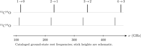
Cataloged rest frequencies for $J=1\to0$ through $4\to3$. Replacing $^{12}\mathrm C$ by $^{13}\mathrm C$ increases the reduced mass and shifts the entire ladder downward. The slight departure from a perfectly scaled, equally spaced comb contains centrifugal-distortion and isotope-dependent effective-structure information. Frequencies are from the JPL Submillimeter, Millimeter, and Microwave Spectral Line Catalog entries 28001 and 29001.

For the $1\to0$ lines,

$$\begin{aligned} \nu_{10}(^{12}\mathrm{CO}) &= 115.2712018\ \mathrm{GHz}, \\ \nu_{10}(^{13}\mathrm{CO}) &= 110.2013541\ \mathrm{GHz}. \end{aligned}$$

Their observed ratio is

$$\frac{\nu_{10}(^{13}\mathrm{CO})} {\nu_{10}(^{12}\mathrm{CO})} = 0.956018.$$

Using isotope mass numbers for a quick rigid estimate gives

$$\begin{aligned} \mu_{12} &\approx \frac{12\times16}{12+16}\,u, \\ \mu_{13} &\approx \frac{13\times16}{13+16}\,u, \end{aligned}$$

and hence

$$\frac{\mu_{12}}{\mu_{13}} = 0.956044.$$

Agreement at roughly $3\times10^{-5}$ is already strong evidence for a common geometry and the expected mass scaling. The residual is meaningful: the $1\to0$ frequency is not exactly $2B$, integer mass numbers are not exact isotopic masses, and $B_0$ contains isotope-dependent zero-point averaging and small non-Born–Oppenheimer corrections.

Isotopic substitution is an assignment test

An isotope pattern contributes several mutually reinforcing checks:

• the frequency shift should have the sign and approximate magnitude predicted from inertia;
• the full set of lines should fit one isotopologue Hamiltonian;
• isotopic abundance should be broadly compatible with signal strength after excitation and dipole factors are included; and
• hyperfine changes should follow the substituted nuclear spin and moments.

One matching line is weak evidence. A coherent mass-scaled ladder is much stronger.

Beyond the diatomic scaling law

For a polyatomic molecule, isotope substitution changes all three principal moments according to the substituted atom’s coordinates relative to the center of mass. The shifts in $A$, $B$, and $C$ are therefore directional. They can help locate the atom in the principal-axis frame, but the axes and center of mass themselves move after substitution. Standard substitution structure formulas account for this geometry; simply attaching $B\propto1/\mu$ to a polyatomic rotor is not valid.

Molecular Structure Determination

Direct result for a diatomic

If $B$ is in ordinary-frequency units, the rigid diatomic relation can be inverted:

$$r = \sqrt{ \frac{h}{8\pi^2\mu B} }.$$

Approximating $B\approx\nu_{10}/2$ and using integer isotope masses in the CO example gives

$$r_{\mathrm{app}} \approx 1.1308\ \text{Å}$$

from either isotopologue. The agreement is the important result; the subscript “app” is equally important. This quick value is based on a ground-state effective constant, not directly on an equilibrium geometry.

Which bond length?

Several structural quantities occur in rotational spectroscopy:

Symbol	Meaning
$r_e$	Equilibrium distance at the minimum of the Born–Oppenheimer potential
$r_0$	Effective ground-vibrational-state structure fitted from ground-state constants
$r_s$	Substitution structure inferred from isotopic moment changes
$r_m$	Mass-dependent fitted structure using several isotopologues
$r_e^{\mathrm{SE}}$	Semi-experimental equilibrium structure after calculated vibrational corrections

These definitions are not interchangeable. A measured $B_0$ reflects a vibrational average of inverse inertia. Even with negligible statistical frequency uncertainty, identifying $B_0$ with $B_e$ leaves a systematic zero-point error.

The polyatomic inverse problem

For nuclei at center-of-mass coordinates $\mathbf r_A$, the inertia tensor is

$$I_{ij} = \sum_A m_A \left( r_A^2\delta_{ij} -r_{A,i}r_{A,j} \right).$$

Diagonalizing it gives $I_a,I_b,I_c$, and hence $A,B,C$. A nonlinear $N$-atom molecule has $3N-6$ internal geometric degrees of freedom, while one isotopologue supplies only three principal moments. Except for very small or strongly constrained molecules, one spectrum cannot determine a unique geometry.

Additional information may come from:

• rotational constants of many singly substituted isotopologues;
• symmetry constraints and known connectivity;
• vibration–rotation corrections from electronic-structure calculations;
• isotopic changes in centrifugal-distortion and hyperfine constants;
• dipole-component information from $a$-, $b$-, and $c$-type intensities;
• independent diffraction, infrared, Raman, or electronic-structure data.

The final geometry should report which data and constraints entered, which parameters were fixed, and how statistical and model uncertainties were propagated.

What dipole components reveal

For an asymmetric top, the appearance of $a$-, $b$-, or $c$-type transitions shows which principal-axis components of the permanent dipole are nonzero. Calibrated relative intensities can constrain $|\mu_a|$, $|\mu_b|$, and $|\mu_c|$ when the populations, line strengths, and instrument response are modeled.

Ordinary field-free intensities do not generally determine the signs of those components. Nor do rotational constants distinguish enantiomers: mirror-image molecules have the same masses and principal moments in an achiral environment. Conformers and constitutional isomers, by contrast, usually have different inertia tensors and can often be separated cleanly.

Precision, accuracy, and identifiability

Three questions should be asked separately:

1. Precision: how reproducibly is each line center measured?
2. Model adequacy: does the effective Hamiltonian predict withheld lines within their uncertainties without structured residuals?
3. Structural identifiability: do the fitted moments and auxiliary data determine the claimed geometry uniquely enough for the stated error bar?

A fit can answer the first question impressively while failing the second or third. More digits in $A$, $B$, and $C$ do not create missing geometric information.

Line Intensities and Temperature

Integrated intensity is the stable object

Peak height changes with broadening even when the number of absorbers and the transition strength do not. For quantitative work, use an integrated absorption coefficient or calibrated emitted intensity with a declared line profile and radiative-transfer model. Absorption and Emission sets out those conventions.

In optically thin thermal absorption, a line intensity is schematically

$$I_{l\to u} \propto N_l S_{lu} |\mu_0|^2 \left[ 1-e^{-h\nu/(k_{\mathrm B}T)} \right],$$

where $S_{lu}$ is the rotational line-strength factor in the chosen normalization. The bracket accounts for stimulated emission. Catalog intensities may fold in partition functions, abundance conventions, and a reference temperature; their documentation is part of the data.

Population diagrams need assumptions

Under optically thin LTE conditions, integrated emission from several transitions can be organized into a rotational diagram. A straight-line form is obtained only after correcting for degeneracy, Einstein coefficients, frequency factors, and beam filling. Curvature can indicate multiple temperatures, optical depth, non-LTE excitation, blends, or inaccurate partition functions. It is not automatically evidence for a new molecular state.

From Peaks to an Assigned Hamiltonian

A defensible assignment workflow is iterative.

1. Calibrate the frequency axis. Record clock traceability, scan linearity, sideband convention, and any frequency multiplication.
2. Characterize the line shape. Distinguish one line from unresolved hyperfine, Doppler doublets, modulation derivatives, and blends.
3. Search for pattern families. Test regular spacing, isotope scaling, spin-statistical alternation, and temperature trends.
4. Propose quantum labels. State whether $J$ or $N$ is used and include $K$, parity, spin, and hyperfine labels as needed.
5. Fit the smallest adequate Hamiltonian. Begin with physically motivated terms and inspect signed residuals, not only a root-mean-square number.
6. Predict unassigned lines. A useful model must forecast transitions outside the fitted subset with credible uncertainties.
7. Confirm independent branches or isotopologues. New line families constrain the assignment far more strongly than extra digits on the same branch.
8. Test experimental controls. Change carrier gas, pressure, discharge, precursor, temperature, polarization, or field where chemically and physically informative.
9. Propagate covariance. Extrapolated line uncertainties depend on parameter correlations and model discrepancy, not just the last printed digit of each constant.
10. Separate the claims. Report observed lines, assigned quantum numbers, fitted spectroscopic constants, and inferred structure as distinct data products.

Using Spectral Catalogs

Catalog entries are evaluated model outputs

The JPL and Cologne databases combine laboratory measurements, effective Hamiltonian fits, and predicted transitions. A typical entry can include frequency, estimated uncertainty, line intensity, lower-state energy, degeneracy, species tag, coding format, and upper and lower quantum numbers. The frequency may be measured directly or predicted from a global fit.

Before using an entry, check:

• the isotopologue, electronic state, vibrational state, and conformer;
• the quantum-number coding and parity convention;
• whether the frequency is measured, fitted, or extrapolated;
• the stated one-standard-deviation uncertainty and its model basis;
• the intensity convention and reference temperature;
• the partition function and nuclear-spin convention; and
• the entry documentation date and cited laboratory data.

An old evaluated entry can remain excellent within its measured range. It should not be treated as current merely because the web interface has a recent date, nor should a low formal uncertainty be trusted far beyond the data that constrain the Hamiltonian.

Database roles

• The JPL Molecular Spectroscopy catalog distributes machine-readable microwave, millimeter-wave, and submillimeter-wave line lists with species-specific documentation.
• The Cologne Database for Molecular Spectroscopy provides evaluated molecular entries and access through astronomical data services.
• The NIST Triatomic Spectral Database explicitly separates observed and predicted frequencies for many triatomics and records uncertainties and literature sources. Its data content was last updated in 2003, so its value is evaluated provenance, not universal recency.

For high-consequence identification or precision work, follow the catalog documentation back to the primary measurements and fitting model.

Common Mistakes

Treating B as Unitless

$B_E$, $B$, and $\widetilde B$ differ by factors of $h$ and $c$. Write the unit on every fitted constant and use $\Delta E=h\nu$, not $\Delta E=\hbar\nu$.

Confusing levels with lines

Rigid-rotor levels scale as $J(J+1)$; adjacent line frequencies scale as $J+1$. Equal line spacing does not mean equal level spacing.

Applying ΔJ = ±1 universally

It is the leading pure rotational E1 rule for the simple linear-rotor case. Asymmetric tops, open-shell states, hyperfine structure, Raman scattering, and field-dressed spectra need additional labels and rules.

Concluding that a nonpolar molecule does not rotate

The permanent-dipole requirement belongs to the E1 transition operator, not to the existence of rotational eigenstates.

Calling B₀ an Equilibrium Constant

$B_0$ includes zero-point vibrational averaging. Recovering $B_e$ and $r_e$ requires vibrational corrections or an explicitly defined alternative structure model.

Inferring a full polyatomic geometry from three constants

$A$, $B$, and $C$ give three principal moments. A general polyatomic geometry has more degrees of freedom and requires isotopologues, constraints, or additional theory.

Fitting every weak feature

Adding distortion constants can absorb blends and misassignments. A term is credible when it improves residual structure, remains stable under data subsets, and predicts new transitions.

Equating peak height with transition strength

Broadening, saturation, modulation, pulse bandwidth, optical depth, and detector response can all change the peak. Compare calibrated integrated quantities under a declared forward model.

Treating a catalog coincidence as identification

Dense spectra contain accidental matches. Confirm multiple transitions with consistent velocity, excitation, isotope behavior, and predicted absences.

Ignoring covariance in extrapolation

Spectroscopic constants are often strongly correlated. Prediction uncertainty must be propagated from the covariance matrix and enlarged when omitted Hamiltonian terms become important.

Key Takeaways

• Pure rotational spectroscopy measures energy differences between molecular rotational states, most often at microwave through submillimeter frequencies.
• A polar linear rigid rotor has $E_J/h=BJ(J+1)$ and leading E1 lines at $\nu_{J+1\leftarrow J}=2B(J+1)$.
• A permanent body-fixed dipole is required for ordinary pure rotational E1 absorption or emission; rotational states exist even when that channel is forbidden.
• Centrifugal distortion and other interactions turn the ideal comb into an effective-Hamiltonian fitting problem.
• Heavier isotope substitution usually lowers rotational frequencies because it increases the moment of inertia.
• Rotational constants determine moments of inertia directly within the fitted model. Molecular geometry requires additional assumptions, isotopologues, and vibrational corrections.
• Catalog frequencies are evaluated data products with conventions, uncertainties, and domains of validity, not context-free measurements.

Exercises

Exercise 1: Unit ledger

A linear molecule has $\widetilde B=1.5000\ \mathrm{cm}^{-1}$. Find its frequency constant $B$ in GHz and the rigid $1\leftarrow0$ transition frequency.

Solution

Using $1\ \mathrm{cm}^{-1}=29.9792458\ \mathrm{GHz}$,

$$\begin{aligned} B &= c\widetilde B \\ &= (29.9792458\ \mathrm{GHz\,cm}) \\ &\quad\times (1.5000\ \mathrm{cm}^{-1}) \\ &= 44.9689\ \mathrm{GHz}. \end{aligned}$$

The rigid $1\leftarrow0$ line is at

$$\nu_1=2B=89.9377\ \mathrm{GHz}.$$

The ordinary frequency, not angular frequency, was used throughout.

Exercise 2: Fit B and D

Two adjacent lines of a semirigid linear rotor are assigned as

$$\begin{gathered} \nu_1=24.999880\ \mathrm{GHz}, \\ \nu_2=49.999040\ \mathrm{GHz}. \end{gathered}$$

Assuming $\nu_n=2Bn-4Dn^3$, determine $B$ and $D$.

Solution

Eliminate $B$:

$$\begin{aligned} D &= \frac{2\nu_1-\nu_2}{24} \\ &= \frac{ 49.999760-49.999040 }{24}\ \mathrm{GHz} \\ &= 0.000030\ \mathrm{GHz} \\ &= 30\ \mathrm{kHz}. \end{aligned}$$

Then

$$\begin{aligned} B &= \frac{\nu_1+4D}{2} \\ &= 12.500000\ \mathrm{GHz}. \end{aligned}$$

A third or higher line is needed to test whether this two-parameter model is adequate.

Exercise 3: Levels without E1 lines

Compare $\mathrm{HCl}$ and $\mathrm N_2$ in their ground electronic and vibrational states. Which has a leading pure rotational electric-dipole spectrum, and does the answer imply that only one molecule has rotational energy levels?

Solution

$\mathrm{HCl}$ has a nonzero permanent dipole and therefore supports the leading E1 $J+1\leftarrow J$ ladder. In field-free $\mathrm N_2$, inversion and exchange symmetry force the permanent electric dipole to vanish, so that E1 ladder is absent.

Both molecules have quantized rotational states. $\mathrm N_2$ rotation can be observed through other operators, including its anisotropic polarizability in rotational Raman scattering.

Exercise 4: Predict an isotope shift

Use mass numbers to estimate the ratio $B(^{13}\mathrm C^{16}\mathrm O)/B(^{12}\mathrm C^{16}\mathrm O)$ under the same-geometry rigid-rotor approximation. Compare it with the measured $1\to0$ frequency ratio $0.956018$.

Solution

The reduced masses in units of $u$ are

$$\mu_{12} = \frac{12\times16}{28}, \qquad \mu_{13} = \frac{13\times16}{29}.$$

Since $B\propto1/\mu$ at fixed geometry,

$$\begin{aligned} \frac{B_{13}}{B_{12}} &\approx \frac{\mu_{12}}{\mu_{13}} \\ &= 0.956044. \end{aligned}$$

The difference from the observed ratio is about

$$2.6\times10^{-5}.$$

It reflects the approximations: integer rather than exact isotopic masses, centrifugal distortion in the $1\to0$ frequencies, isotope-dependent vibrational averaging, and smaller non-Born–Oppenheimer effects.

Exercise 5: Most populated level

A linear rotor has $B=10.0\ \mathrm{GHz}$ and is in thermal equilibrium at $T=20.0\ \mathrm K$. Ignoring nuclear-spin weights, estimate the most populated $J$. Use $k_{\mathrm B}/h=20.8366\ \mathrm{GHz\,K^{-1}}$. Why does this not by itself locate the strongest absorption line?

Solution

The continuous estimate gives

$$\begin{aligned} J_{\mathrm{pop}} &\approx \frac12 \left[ \sqrt{ \frac{2(20.8366)(20.0)}{10.0} } -1 \right] \\ &\approx 4.06. \end{aligned}$$

The most populated integer level is therefore expected near $J=4$; exact discrete populations should be compared around that value.

The strongest absorption line also depends on the $J\to J+1$ line-strength factor, the stimulated-emission correction, frequency dependence, broadening, abundance, optical depth, and instrument response. The population maximum is only one input.

Exercise 6: Structural identifiability

One isotopologue of a nonlinear six-atom molecule has accurately fitted $A_0,B_0,C_0$. Explain why these constants do not uniquely determine all equilibrium bond lengths and angles.

Solution

A nonlinear six-atom molecule has

$$3N-6=12$$

internal geometric degrees of freedom. The three rotational constants supply three principal moments of inertia, so the inverse problem is underdetermined. In addition, the subscript $0$ denotes ground-state vibrational averaging rather than equilibrium moments.

Multiple isotopologues, symmetry and connectivity constraints, and computed vibration–rotation corrections are typical additional inputs. Their assumptions must be included in any structural uncertainty.

Exercise 7: Catalog coincidence and Doppler velocity

An astronomical feature appears at $99.9960\ \mathrm{GHz}$ near a catalog rest frequency of $100.0000\ \mathrm{GHz}$. Using the nonrelativistic radio sign convention, estimate the recession velocity. Why is this one match not enough for a molecular identification?

Solution

With $v_r>0$ for recession,

$$\frac{\nu_{\mathrm{obs}}-\nu_0}{\nu_0} \approx -\frac{v_r}{c}.$$

Therefore

$$\begin{aligned} v_r &\approx c\frac{\nu_0-\nu_{\mathrm{obs}}}{\nu_0} \\ &= c(4.0\times10^{-5}) \\ &\approx 12.0\ \mathrm{km\,s^{-1}}. \end{aligned}$$

Dense line surveys contain accidental frequency coincidences. A credible identification should reproduce several transitions at the same velocity with compatible excitation, width, spatial distribution, isotope behavior, and predicted non-detections.

Exercise 8: Extrapolation test

A fit to low-$J$ lines has a small residual using only $B$ and $D$. At high $J$, all observed lines lie progressively above the predictions. Give two possible explanations and one test that distinguishes a random measurement error from model inadequacy.

Solution

Possible physical explanations include a missing sextic distortion term $H$, interaction with a nearby state, or a high-$J$ assignment error. A frequency-calibration error that changes with band is another systematic possibility.

Random independent errors should fluctuate in sign. A smooth, quantum-number dependent sequence of signed residuals is evidence of model inadequacy or a correlated calibration problem. Fit and withhold interleaved high-$J$ lines, inspect residuals versus $J$ and frequency band, and test whether one physically motivated extra term predicts the withheld data. Merely reducing the residual on the fitted points is insufficient.

Cross-Links

• Spectroscopy Nomenclature decodes O, P, Q, R, and S branches, lower-state parenthetical labels, and compound branch strings when both $N$ and $J$ are resolved.
• Spectroscopy
• Transition Rates
• Selection Rules in Spectroscopy
• Line Shapes and Broadening
• Absorption and Emission
• Vibrational Spectroscopy
• Raman Spectroscopy
• Rotations of Molecules
• Rovibrational Coupling
• Molecular Symmetry
• Rigid Rotor
• Rotational Spectra
• Rotor in External Fields: First Encounter
• Applications to Molecular Rotations
• Selection Rules
• Selection Rule Tables for rotational and rovibrational branch rules

References

• International Union of Pure and Applied Chemistry, “rotational constant”, Compendium of Chemical Terminology, 5th ed., online version 5.0.0, 2025.
• C. H. Townes and A. L. Schawlow, Microwave Spectroscopy, McGraw–Hill, 1955; Dover reprint, 1975.
• W. Gordy and R. L. Cook, Microwave Molecular Spectra, 3rd ed., Wiley, 1984.
• J. M. Brown and A. Carrington, Rotational Spectroscopy of Diatomic Molecules, Cambridge University Press, 2003, doi:10.1017/CBO9780511814808.
• P. F. Bernath, Spectra of Atoms and Molecules, 5th ed., Oxford University Press, 2025, doi:10.1093/oso/9780197754498.001.0001.
• H. M. Pickett, “The Fitting and Prediction of Vibration-Rotation Spectra with Spin Interactions,” Journal of Molecular Spectroscopy 148, 371–377 (1991), doi:10.1016/0022-2852(91)90293-O.
• H. M. Pickett, R. L. Poynter, E. A. Cohen, M. L. Delitsky, J. C. Pearson, and H. S. P. Müller, “Submillimeter, Millimeter, and Microwave Spectral Line Catalog,” Journal of Quantitative Spectroscopy and Radiative Transfer 60, 883–890 (1998), doi:10.1016/S0022-4073(98)00091-0.
• H. S. P. Müller, S. Thorwirth, D. A. Roth, and G. Winnewisser, “The Cologne Database for Molecular Spectroscopy, CDMS,” Astronomy & Astrophysics 370, L49–L52 (2001), doi:10.1051/0004-6361:20010367.
• C. P. Endres, S. Schlemmer, P. Schilke, J. Stutzki, and H. S. P. Müller, “The Cologne Database for Molecular Spectroscopy, CDMS, in the Virtual Atomic and Molecular Data Centre, VAMDC,” Journal of Molecular Spectroscopy 327, 95–104 (2016), doi:10.1016/j.jms.2016.03.005.
• NIST Physical Measurement Laboratory, Triatomic Spectral Database, Standard Reference Database 117, data content updated July 2003, doi:10.18434/T4DW2S, accessed 2026-07-22.
• JPL Molecular Spectroscopy, $^{12}\mathrm C^{16}\mathrm O$ catalog entry 28001 and $^{13}\mathrm C^{16}\mathrm O$ catalog entry 29001, accessed 2026-07-22.
• J. Kraitchman, “Determination of Molecular Structure from Microwave Spectroscopic Data,” American Journal of Physics 21, 17–24 (1953), doi:10.1119/1.1933338.
• C. C. Costain, “Determination of Molecular Structures from Ground State Rotational Constants,” Journal of Chemical Physics 29, 864–874 (1958), doi:10.1063/1.1744602.