Einstein Coefficients

Einstein coefficients package three weak-field radiative processes between a lower level $1$ and an upper level $2$:

$$\begin{aligned} R_{1\rightarrow2} &= B_{12}^{(\omega)} u_\omega(\omega_0), \\ R_{2\rightarrow1} &= A_{21} + B_{21}^{(\omega)} u_\omega(\omega_0). \end{aligned}$$

Here

$$\hbar\omega_0=E_2-E_1>0.$$

The three terms describe:

• absorption, proportional to $B_{12}^{(\omega)}$;
• stimulated emission, proportional to $B_{21}^{(\omega)}$;
• spontaneous emission, proportional to $A_{21}$.

The superscript $(\omega)$ is not decorative. It declares that $u_\omega(\omega)$ is the total isotropic radiation energy density per unit angular frequency, summed over propagation directions and polarizations. A different spectral variable changes the numerical $B$ coefficient.

The $A$ coefficient is a rate. A $B$ coefficient is not: it becomes a rate only after multiplication by the matching spectral energy density. Neither coefficient is a finite-time Born-rule probability.

Canonical Scope

This page owns the spectroscopy-facing definitions of the Einstein $A$ and $B$ coefficients, the detailed-balance derivation of their relations, their connection to Planck radiation, and the convention ledger needed to compare tabulated or calculated values.

Several nearby pages keep narrower canonical responsibilities:

• Transition Rates in Light–Matter Interaction owns the microscopic mode-quantization derivation of absorption, stimulated emission, and spontaneous emission, including the bosonic $n$ and $n+1$ factors.
• Spontaneous Emission owns Wigner–Weisskopf decay, lifetime and natural linewidth, angular emission, photon wavepackets, and structured-environment modification.
• Transition Rates owns the general distinction among probabilities, rates, cross sections, populations, and detector signals.
• Oscillator Strengths owns dimensionless E1 strengths, sum rules, and integrated absorption.
• Planck’s Radiation Law owns the historical and modern blackbody-spectrum derivations.
• Optical Bloch Equations owns coherent driving with relaxation, dephasing, saturation, and steady-state response.
• Quantum Optical Master Equation owns open-system dynamics in vacuum and thermal photon reservoirs.

The Einstein picture is a rate model for weak, incoherent radiation and population kinetics. It is not a replacement for coherent amplitudes, strong-drive dynamics, or environment-specific quantum electrodynamics.

Convention Ledger

Unless stated otherwise:

• $E_2>E_1$ and $\omega_0=(E_2-E_1)/\hbar$;
• $g_1$ and $g_2$ are the degeneracies of the lower and upper levels;
• $N_1$ and $N_2$ are populations or number densities of those levels;
• populations within each degenerate level are uniformly distributed;
• $u_\omega(\omega)$ is total isotropic vacuum radiation energy per volume per unit angular frequency;
• all propagation directions and both transverse polarizations are included in $u_\omega$;
• the line is sufficiently narrow that the radiation density can be evaluated at $\omega_0$;
• the radiation is weak enough for rates to remain linear in spectral energy density;
• coefficients refer to one declared radiative channel or to an explicitly stated sum of channels.

The simple Einstein relations concern sharp levels in thermal equilibrium. Broad molecular bands, overlapping lines, anisotropic reservoirs, polarization-selected transitions, and structured photonic environments require more detailed spectral or mode-resolved descriptions.

A and B Coefficients

Spontaneous-emission coefficient A

The coefficient $A_{21}$ is the spontaneous transition rate per system prepared in level $2$ for the specified downward radiative channel:

$$A_{21} = \left. \frac{dP_{2\rightarrow1}}{dt} \right|_{\mathrm{sp}}, \qquad [A_{21}]=\mathrm{s}^{-1}.$$

For a population $N_2$, the expected number of photons emitted into that channel per unit time is

$$\dot N_{\gamma,21} = N_2A_{21}$$

when reabsorption, stimulated processes, and detector effects are excluded. The corresponding emitted power is

$$\mathcal P_{21} = N_2\hbar\omega_0A_{21}.$$

Atomic databases often call $A_{21}$ a transition probability, but its units show that it is a probability rate, not a dimensionless probability.

Radiative lifetime and branching

If upper level $2$ can decay radiatively to several lower levels $\ell$, its total radiative width in inverse-time units is

$$\Gamma_{\mathrm{rad},2} = \sum_\ell A_{2\ell}.$$

The radiative lifetime is

$$\tau_{\mathrm{rad},2} = \frac{1}{\Gamma_{\mathrm{rad},2}}.$$

The radiative branching fraction into channel $2\rightarrow1$ is

$$b_{21}^{(\mathrm{rad})} = \frac{A_{21}} {\sum_\ell A_{2\ell}}.$$

If nonradiative, collisional, predissociative, or quenching channels are present,

$$\Gamma_{\mathrm{tot},2} = \Gamma_{\mathrm{rad},2} + \Gamma_{\mathrm{nr},2} + \Gamma_{\mathrm{coll},2} + \cdots,$$

and

$$\tau_{\mathrm{obs},2} = \frac{1}{\Gamma_{\mathrm{tot},2}}.$$

The radiative quantum yield is

$$\Phi_{\mathrm{rad}} = \frac{\Gamma_{\mathrm{rad},2}} {\Gamma_{\mathrm{tot},2}}.$$

Thus one $A$ coefficient, a radiative lifetime, an observed lifetime, and a fluorescence quantum yield are four different quantities.

Stimulated coefficients B

The coefficient $B_{12}^{(\omega)}$ converts spectral energy density into an absorption rate:

$$R_{1\rightarrow2}^{(\mathrm{abs})} = B_{12}^{(\omega)} u_\omega(\omega_0).$$

Similarly,

$$R_{2\rightarrow1}^{(\mathrm{stim})} = B_{21}^{(\omega)} u_\omega(\omega_0).$$

In SI units,

$$\left[ u_\omega \right] = \mathrm{J\,m^{-3}} \left(\mathrm{rad\,s^{-1}}\right)^{-1},$$

so, treating radians as dimensionless,

$$\left[ B^{(\omega)} \right] = \mathrm{m^3\,J^{-1}\,s^{-2}}.$$

Only the products $B_{12}^{(\omega)}u_\omega$ and $B_{21}^{(\omega)}u_\omega$ have dimensions of inverse time.

Finite line profiles

For a normalized absorption profile,

$$\int_0^\infty \phi_{12}^{(\omega)}(\omega)\,d\omega =1,$$

the weak-field rate is more generally

$$R_{1\rightarrow2}^{(\mathrm{abs})} = B_{12}^{(\omega)} \int_0^\infty u_\omega(\omega) \phi_{12}^{(\omega)}(\omega)\,d\omega.$$

If $u_\omega$ varies negligibly across the line, this reduces to

$$R_{1\rightarrow2}^{(\mathrm{abs})} \simeq B_{12}^{(\omega)} u_\omega(\omega_0).$$

For spontaneous emission, a normalized profile can distribute the total coefficient:

$$\begin{aligned} \frac{dA_{21}}{d\omega} &= A_{21} \phi_{21}^{(\omega)}(\omega), \\ \int_0^\infty \frac{dA_{21}}{d\omega}\,d\omega &= A_{21}. \end{aligned}$$

The integrated coefficient and the spectral line shape are separate inputs. For broad vibronic bands, absorption and emission profiles need not be identical, and the sharp-line detailed-balance derivation below should not be applied point by point without additional assumptions.

Ordinary frequency versus angular frequency

Let $u_\nu(\nu)$ be energy density per unit ordinary frequency. Conservation of energy in a spectral interval requires

$$u_\nu(\nu)\,d\nu = u_\omega(\omega)\,d\omega.$$

Because

$$\omega=2\pi\nu, \qquad d\omega=2\pi\,d\nu,$$

the densities satisfy

$$u_\nu(\nu) = 2\pi u_\omega(\omega).$$

The same physical rate can be written

$$B_{ij}^{(\nu)}u_\nu = B_{ij}^{(\omega)}u_\omega,$$

so

$$B_{ij}^{(\nu)} = \frac{1}{2\pi} B_{ij}^{(\omega)}.$$

An unlabeled $B_{ij}$ is therefore incomplete. The factors of $2\pi$ cannot be repaired by dimensional analysis because the two $B$ conventions have the same SI dimensions when radians are treated as dimensionless.

Energy density is not beam intensity

Einstein’s thermal argument uses isotropic spectral energy density. For isotropic specific intensity $I_\nu$,

$$u_\nu = \frac{4\pi}{c} I_\nu.$$

A collimated polarized laser beam is not isotropic. Its irradiance, polarization, propagation direction, and coherence must be converted to the field quantity appropriate to the transition. In coherent spectroscopy, a Rabi frequency or optical Bloch description is usually clearer than inserting beam intensity into $B u$ as though it were an isotropic blackbody density.

Detailed Balance

Thermal level populations

At temperature $T$, thermal equilibrium gives

$$\frac{N_2}{N_1} = \frac{g_2}{g_1} \exp\left( -\frac{\hbar\omega_0}{k_{\mathrm B}T} \right).$$

Define

$$\beta = \frac{1}{k_{\mathrm B}T}.$$

The ratio can then be written

$$\frac{N_2}{N_1} = \frac{g_2}{g_1} e^{-\beta\hbar\omega_0}.$$

The degeneracies matter because thermal equilibrium populates individual microstates according to Boltzmann weights. A level with more substates has a larger total population at the same energy per substate.

Balance of upward and downward events

At equilibrium, the total upward transition count equals the total downward count:

$$N_1B_{12}^{(\omega)}u_\omega = N_2 \left[ A_{21} + B_{21}^{(\omega)}u_\omega \right].$$

Solving for the equilibrium radiation density gives

$$u_\omega = \frac{A_{21}} { \dfrac{N_1}{N_2} B_{12}^{(\omega)} - B_{21}^{(\omega)} }.$$

Using the Boltzmann population ratio,

$$u_\omega = \frac{A_{21}} { \dfrac{g_1}{g_2} B_{12}^{(\omega)} e^{\beta\hbar\omega_0} - B_{21}^{(\omega)} }.$$

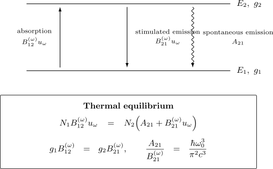
Einstein’s three-process rate model for two sharp levels in an isotropic radiation field. Thermal equilibrium fixes the degeneracy relation between the two stimulated coefficients and the ratio of spontaneous to stimulated emission coefficients.

Matching Planck’s law

The blackbody energy density per unit angular frequency is

$$u_\omega(\omega,T) = \frac{\hbar\omega^3} {\pi^2c^3} \frac{1} {e^{\beta\hbar\omega}-1}.$$

For the rate-balance expression to have this form at every temperature, the coefficients must obey

$$g_1B_{12}^{(\omega)} = g_2B_{21}^{(\omega)}$$

and

$$\frac{A_{21}} {B_{21}^{(\omega)}} = \frac{\hbar\omega_0^3} {\pi^2c^3}.$$

In ordinary-frequency notation, the same relations are

$$g_1B_{12}^{(\nu)} = g_2B_{21}^{(\nu)}$$

and

$$\frac{A_{21}} {B_{21}^{(\nu)}} = \frac{8\pi h\nu_0^3} {c^3}.$$

The two $A/B$ formulas are physically equivalent. Their different numerical prefactors follow entirely from the definitions of spectral density and $B$.

What equilibrium does and does not determine

Thermodynamic balance determines:

• the ratio of absorption to stimulated-emission coefficients after degeneracies are included;
• the ratio of spontaneous to stimulated-emission coefficients after the radiation-density convention is fixed.

It does not determine the absolute magnitude of $A_{21}$ or $B_{21}^{(\omega)}$. That magnitude depends on the transition matrix element. Modern quantum electrodynamics supplies it microscopically.

The first relation is sometimes written $B_{12}=B_{21}$. That is correct for two nondegenerate states or for matched state-to-state coefficients. For level-averaged coefficients,

$$B_{12}^{(\omega)} = \frac{g_2}{g_1} B_{21}^{(\omega)}.$$

Ignoring this distinction is a common source of factors $2J+1$.

Microscopic reversibility

For resolved substates connected by the same polarization component, the Hermiticity of the interaction gives equal squared forward and reverse matrix elements. Level-averaged absorption sums over final substates while stimulated emission averages over a different initial manifold. Counting those substates produces

$$g_1B_{12}=g_2B_{21}.$$

The degeneracy relation is therefore consistent with microscopic reversibility; it does not assert that the two level-averaged numbers must be equal.

Blackbody Radiation Connection

Photon occupation form

The thermal mean occupation of a photon mode is

$$\overline n(\omega,T) = \frac{1} {e^{\beta\hbar\omega}-1}.$$

Planck’s angular-frequency energy density can be factored as

$$u_\omega(\omega,T) = u_0^{(\omega)}(\omega) \overline n(\omega,T),$$

where

$$u_0^{(\omega)}(\omega) = \frac{\hbar\omega^3} {\pi^2c^3}.$$

This is a convenient free-space mode-density scale, not the divergent zero-point energy density of the electromagnetic vacuum. At the transition frequency it is precisely the ratio

$$u_0^{(\omega)}(\omega_0) = \frac{A_{21}} {B_{21}^{(\omega)}}.$$

It converts the spontaneous rate to the stimulated coefficient.

Thermal upward and downward rates

Using the Einstein relations,

$$B_{21}^{(\omega)} u_\omega(\omega_0,T) = A_{21} \overline n(\omega_0,T).$$

Thus the downward rate per system in level $2$ is

$$R_{2\rightarrow1}^{(\mathrm{th})} = A_{21} \left[ \overline n(\omega_0,T)+1 \right].$$

The upward rate per system in level $1$ is

$$R_{1\rightarrow2}^{(\mathrm{th})} = \frac{g_2}{g_1} A_{21} \overline n(\omega_0,T).$$

For equal degeneracies, these reduce to the familiar quantum-optical expressions proportional to $\overline n$ and $\overline n+1$.

The identity

$$\overline n+1 = e^{\beta\hbar\omega_0} \overline n$$

ensures that the Boltzmann population ratio makes total upward and downward event counts equal.

Low- and high-temperature limits

When

$$\hbar\omega_0\gg k_{\mathrm B}T,$$

the occupation is

$$\overline n \simeq e^{-\beta\hbar\omega_0}\ll1.$$

Stimulated processes from a thermal field are then negligible compared with spontaneous emission. This is typical for visible transitions at room temperature.

When

$$\hbar\omega_0\ll k_{\mathrm B}T,$$

the occupation is

$$\overline n \simeq \frac{k_{\mathrm B}T} {\hbar\omega_0}\gg1.$$

Stimulated emission and absorption dominate over the extra spontaneous $+1$. Microwave and radio-frequency transitions can therefore be strongly affected by thermal photons even at ordinary laboratory temperatures.

The stimulated and spontaneous downward contributions are equal when

$$\overline n=1,$$

or

$$T = \frac{\hbar\omega_0} {k_{\mathrm B}\ln 2}.$$

Historical logic

Einstein introduced the three-process rate structure in 1916–1917 and used thermal equilibrium with the known radiation law to constrain the coefficients. Stimulated emission emerged as a necessary process: absorption and spontaneous emission alone cannot reproduce Planck’s denominator.

The argument was extraordinarily predictive, but it was not yet a modern quantized-field calculation of $A_{21}$. Dirac’s 1927 radiation theory and later quantum electrodynamics supplied a microscopic account of emission and absorption amplitudes. The historical development should not be compressed into the claim that equilibrium thermodynamics alone calculated every coefficient.

Relation to Transition Dipole Moments

Nondegenerate E1 transition

For a nondegenerate electric-dipole transition in vacuum, define

$$\mathbf d_{21} = \langle2| \widehat{\mathbf D} |1\rangle.$$

The free-space spontaneous-emission coefficient is

$$A_{21} = \frac{\omega_0^3} {3\pi\epsilon_0\hbar c^3} \left| \mathbf d_{21} \right|^2.$$

Combining this with the angular-frequency Einstein relation gives

$$B_{21}^{(\omega)} = \frac{\pi} {3\epsilon_0\hbar^2} \left| \mathbf d_{21} \right|^2.$$

For two nondegenerate states,

$$B_{12}^{(\omega)} = B_{21}^{(\omega)}.$$

In ordinary-frequency notation,

$$B_{21}^{(\nu)} = \frac{1}{6\epsilon_0\hbar^2} \left| \mathbf d_{21} \right|^2.$$

These equations display the convention dependence directly:

$$B_{21}^{(\omega)} = 2\pi B_{21}^{(\nu)}.$$

Degenerate angular-momentum levels

For an E1 transition between levels with reduced line strength

$$S_{21} = \left| \left\langle \gamma_2J_2 \left\| \widehat D^{(1)} \right\| \gamma_1J_1 \right\rangle \right|^2,$$

the level-averaged coefficients are

$$\begin{aligned} A_{21} &= \frac{\omega_0^3} {3\pi\epsilon_0\hbar c^3g_2} S_{21}, \\ B_{21}^{(\omega)} &= \frac{\pi} {3\epsilon_0\hbar^2g_2} S_{21}, \\ B_{12}^{(\omega)} &= \frac{\pi} {3\epsilon_0\hbar^2g_1} S_{21}. \end{aligned}$$

The first coefficient averages over upper substates; the absorption coefficient averages over lower substates. The common reduced line strength makes the degeneracy relation manifest.

Relation to oscillator strength

For an E1 absorption oscillator strength $f_{12}$,

$$A_{21} = \frac{e^2\omega_0^2} {2\pi\epsilon_0m_ec^3} \frac{g_1}{g_2} f_{12}.$$

The stimulated coefficients are

$$\begin{aligned} B_{12}^{(\omega)} &= \frac{\pi e^2} {2\epsilon_0m_e\hbar\omega_0} f_{12}, \\ B_{21}^{(\omega)} &= \frac{g_1}{g_2} B_{12}^{(\omega)}. \end{aligned}$$

The complete convention and line-strength ledger belongs to Oscillator Strengths.

Frequency scaling

For a fixed transition dipole,

$$A_{21}\propto\omega_0^3, \qquad B_{21}^{(\omega)} \propto \left|\mathbf d_{21}\right|^2.$$

The spontaneous rate carries the free-space photon mode-density factor $\omega_0^2$ and one additional frequency from field normalization. The angular-frequency $B$ coefficient does not carry that $\omega_0^3$ factor. The relation

$$\frac{A_{21}} {B_{21}^{(\omega)}} \propto \omega_0^3$$

therefore reflects the available free-space radiation modes, not a temperature dependence of either intrinsic coefficient.

Beyond electric dipole and free space

Einstein $A$ coefficients are also tabulated for M1, E2, and higher-multipole transitions, but their microscopic line-strength formulas differ from the E1 expressions above. The equilibrium $A/B$ relation for a sharp one-photon transition still relies on the declared radiation-mode convention.

In a cavity, waveguide, dielectric, near a surface, or in another structured photonic environment, spontaneous emission depends on the local electromagnetic density of states and field mode functions. The free-space formula can be enhanced, suppressed, or made anisotropic. One should then use an environment-specific mode sum or electromagnetic Green tensor rather than silently reusing the vacuum $A_{21}$. See Spontaneous Emission for the Green-tensor and Purcell-factor preview.

Link to Lasers and Spontaneous Emission

Net stimulated gain

In a radiation field, the net stimulated downward event rate per volume is

$$\begin{aligned} \mathcal R_{\mathrm{stim,net}} &= N_2B_{21}^{(\omega)}u_\omega - N_1B_{12}^{(\omega)}u_\omega \\ &= B_{21}^{(\omega)}u_\omega \left( N_2 - \frac{g_2}{g_1}N_1 \right). \end{aligned}$$

Net gain requires

$$\frac{N_2}{g_2} > \frac{N_1}{g_1}.$$

This is population inversion per substate. The simpler condition $N_2>N_1$ is sufficient only when $g_1=g_2$.

A thermal two-level ensemble cannot satisfy this inequality because

$$\frac{N_2/g_2}{N_1/g_1} = e^{-\beta\hbar\omega_0} <1.$$

Pumping and additional levels are therefore needed to maintain inversion in a laser medium.

Role of spontaneous emission

Spontaneous emission:

• depletes the upper laser level;
• seeds photons with random emission times, directions, phases, and polarizations;
• contributes quantum noise;
• competes with nonradiative decay and cavity loss;
• supplies fluorescence even below threshold.

Stimulated emission into a selected mode copies that mode’s frequency, polarization, propagation direction, and phase relation. The Einstein rate picture captures population transfer and small-signal gain, but a coherent laser field and its phase dynamics require Maxwell–Bloch, master-equation, or quantum-optical methods.

When rate equations fail

The Einstein equations assume that optical coherence can be neglected and that transition events can be described by approximately constant rates. They become inadequate when:

• a coherent pulse drives resolved Rabi oscillations;
• the field is strong enough to saturate or power broaden the transition;
• coherence between degenerate substates matters;
• one cavity mode exchanges excitations reversibly with the emitter;
• reservoir memory or strong light–matter coupling invalidates Markovian decay;
• interference among multiple pathways changes the transition amplitude.

The appropriate coherent two-level treatment is developed in Optical Bloch Equations.

Spontaneous emission is not classical driving

A prescribed classical field can produce absorption and stimulated emission, but it does not derive spontaneous emission from an initially empty field. In the quantized-field description, downward coupling to a photon mode has the matrix-element factor

$$\sqrt{n+1},$$

while absorption has

$$\sqrt n.$$

The surviving unity at $n=0$, summed over vacuum modes, produces the spontaneous rate. The full derivation and free-space dipole radiation pattern belong to Transition Rates in Light–Matter Interaction.

Common Mistakes

Quoting B without its spectral convention

$B^{(\nu)}$ and $B^{(\omega)}$ differ by $2\pi$. Additional conventions may use energy per solid angle, per polarization, or per wavenumber. State the field density explicitly.

Treating B as a rate

$B$ requires multiplication by a compatible spectral energy density. Its units are not inverse seconds.

Setting B12 equal to B21 for degenerate levels

State-to-state coefficients can be equal, but level-averaged coefficients obey $g_1B_{12}=g_2B_{21}$.

Calling A a dimensionless probability

$A_{21}$ is a rate. Over a sufficiently short rate interval,

$$P_{2\rightarrow1}(t) \simeq A_{21}t,$$

but the exact finite-time probability and depletion law require a dynamical model.

Confusing radiative and observed lifetimes

The inverse observed lifetime contains all decay channels. It equals $\sum_\ell A_{2\ell}$ only when nonradiative and collisional losses are negligible.

Inserting beam irradiance into an isotropic formula

Irradiance, radiance, energy density, and spectral energy density are different quantities. Directional polarization coupling cannot be recovered from total isotropic $u_\omega$ after the information has been discarded.

Assuming equilibrium fixes absolute strengths

Detailed balance fixes coefficient ratios. A matrix element or measured quantity is needed to determine their absolute scale.

Using free-space A in a structured reservoir

Cavities, interfaces, and photonic materials modify the available modes. Their emission rates are not universal properties of the isolated emitter alone.

Applying rate equations to coherent strong driving

When phase coherence, Rabi cycling, or saturation matters, use amplitudes, density matrices, or optical Bloch equations.

Practical Workflow

When using Einstein coefficients:

1. identify the lower and upper levels and their degeneracies;
2. declare whether the coefficients are state-resolved, level-averaged, or multiplet-averaged;
3. specify ordinary frequency, angular frequency, wavelength, wavenumber, or another spectral coordinate;
4. define whether the field density includes all directions and polarizations;
5. normalize any absorption and emission profiles;
6. distinguish one $A$ channel from the sum controlling a lifetime;
7. include nonradiative, collisional, transfer, and reabsorption processes when comparing with measured kinetics;
8. use dipole moments, line strengths, oscillator strengths, and database values only after matching degeneracy and unit conventions;
9. replace the rate model by coherent or environment-specific dynamics when its assumptions fail.

Key Takeaways

• $A_{21}$ is a spontaneous-emission rate; $B_{ij}$ becomes a stimulated rate only after multiplication by a matching spectral energy density.
• The numerical value of a $B$ coefficient depends on the spectral-density convention.
• Level-averaged coefficients satisfy $g_1B_{12}=g_2B_{21}$.
• In the angular-frequency convention, $A_{21}/B_{21}^{(\omega)}=\hbar\omega_0^3/(\pi^2c^3)$.
• The same relations reproduce Planck’s law in thermal equilibrium but do not determine the absolute transition strength.
• Free-space E1 coefficients are fixed by one transition dipole or reduced line strength.
• Radiative lifetime requires a sum over all spontaneous channels; measured lifetime can include additional losses.
• Laser gain requires inversion per degenerate substate, not merely more particles in the upper level.
• Strong coherent driving and structured reservoirs lie beyond the simple Einstein rate model.

Exercises

Exercise 1: Convert B between spectral conventions

Show that

$$B_{21}^{(\nu)} = \frac{B_{21}^{(\omega)}}{2\pi}$$

when $u_\nu$ and $u_\omega$ describe the same radiation field. Verify that the stimulated rate is unchanged.

Solution

The spectral energy in a physical interval is invariant:

$$u_\nu\,d\nu = u_\omega\,d\omega.$$

Since $d\omega=2\pi\,d\nu$,

$$u_\nu=2\pi u_\omega.$$

Rate invariance requires

$$B_{21}^{(\nu)}u_\nu = B_{21}^{(\omega)}u_\omega.$$

Substitution gives

$$B_{21}^{(\nu)} (2\pi u_\omega) = B_{21}^{(\omega)}u_\omega,$$

and therefore

$$B_{21}^{(\nu)} = \frac{B_{21}^{(\omega)}}{2\pi}.$$

The coefficient and density change inversely, leaving their product unchanged.

Exercise 2: Derive the Einstein relations

Starting from thermal population balance and Planck’s angular-frequency energy density, derive the two Einstein relations for levels with degeneracies $g_1$ and $g_2$.

Solution

Equilibrium requires

$$N_1B_{12}^{(\omega)}u_\omega = N_2 \left( A_{21} + B_{21}^{(\omega)}u_\omega \right).$$

With

$$\frac{N_2}{N_1} = \frac{g_2}{g_1} e^{-\beta\hbar\omega_0},$$

solving for $u_\omega$ gives

$$u_\omega = \frac{A_{21}} { \dfrac{g_1}{g_2} B_{12}^{(\omega)} e^{\beta\hbar\omega_0} - B_{21}^{(\omega)} }.$$

To match a denominator proportional to $e^{\beta\hbar\omega_0}-1$, require

$$\frac{g_1}{g_2} B_{12}^{(\omega)} = B_{21}^{(\omega)}.$$

Hence

$$g_1B_{12}^{(\omega)} = g_2B_{21}^{(\omega)}.$$

The remaining prefactor must match Planck’s law:

$$\frac{A_{21}} {B_{21}^{(\omega)}} = \frac{\hbar\omega_0^3} {\pi^2c^3}.$$

Exercise 3: Degenerate levels

An E1 line connects

$$J_1=\frac{1}{2}, \qquad J_2=\frac{3}{2}.$$

Find $B_{12}^{(\omega)}/B_{21}^{(\omega)}$ for level-averaged coefficients.

Solution

The statistical weights are

$$\begin{aligned} g_1&=2J_1+1=2, \\ g_2&=2J_2+1=4. \end{aligned}$$

Detailed balance gives

$$g_1B_{12}^{(\omega)} = g_2B_{21}^{(\omega)}.$$

Therefore

$$\frac{B_{12}^{(\omega)}} {B_{21}^{(\omega)}} = \frac{g_2}{g_1} =2.$$

This factor does not violate microscopic reversibility. It arises because the absorption coefficient averages over two lower substates while the stimulated-emission coefficient averages over four upper substates.

Exercise 4: Thermal photons at optical and microwave frequencies

Evaluate the thermal occupation

$$\overline n = \frac{1}{e^{h\nu/(k_{\mathrm B}T)}-1}$$

at $T=300\ \mathrm K$ for:

1. $\nu=5.00\times10^{14}\ \mathrm{Hz}$;
2. $\nu=1.00\times10^{10}\ \mathrm{Hz}$.

Interpret the ratio of stimulated to spontaneous downward rates.

Solution

For the optical transition,

$$\frac{h\nu}{k_{\mathrm B}T} \simeq 79.99,$$

so

$$\overline n_{\mathrm{opt}} \simeq 1.83\times10^{-35}.$$

Thermal stimulated emission is negligible compared with spontaneous emission.

For the microwave transition,

$$\frac{h\nu}{k_{\mathrm B}T} \simeq 1.600\times10^{-3},$$

so

$$\overline n_{\mathrm{mw}} \simeq 6.25\times10^2.$$

Because

$$\frac{R_{\mathrm{stim}}}{R_{\mathrm{sp}}} = \overline n,$$

thermal stimulated emission dominates for the microwave transition. The same thermal field also drives strong absorption.

Exercise 5: Lifetime, branching, and quantum yield

An upper level has two radiative channels,

$$\begin{aligned} A_{21}&=2.0\times10^7\ \mathrm{s}^{-1}, \\ A_{20}&=6.0\times10^7\ \mathrm{s}^{-1}, \end{aligned}$$

and a nonradiative decay rate

$$\Gamma_{\mathrm{nr}} = 2.0\times10^7\ \mathrm{s}^{-1}.$$

Find the radiative lifetime, observed lifetime, radiative quantum yield, and the total-event branching probabilities.

Solution

The radiative rate is

$$\Gamma_{\mathrm{rad}} = A_{21}+A_{20} = 8.0\times10^7\ \mathrm{s}^{-1},$$

so

$$\tau_{\mathrm{rad}} = 12.5\ \mathrm{ns}.$$

The total rate is

$$\Gamma_{\mathrm{tot}} = 1.0\times10^8\ \mathrm{s}^{-1},$$

giving

$$\tau_{\mathrm{obs}} = 10.0\ \mathrm{ns}.$$

The radiative quantum yield is

$$\Phi_{\mathrm{rad}} = \frac{8.0\times10^7}{1.0\times10^8} =0.80.$$

The probabilities that a decay event uses the three channels are

$$\begin{aligned} p_{21}&=0.20, \\ p_{20}&=0.60, \\ p_{\mathrm{nr}}&=0.20. \end{aligned}$$

Conditioned on a radiative event, the two radiative branching fractions are $0.25$ and $0.75$.

Exercise 6: A coefficient from a transition dipole

A nondegenerate E1 transition in vacuum has

$$\lambda=500\ \mathrm{nm}, \qquad \left|\mathbf d_{21}\right| = ea_0.$$

Estimate $A_{21}$ and the single-channel radiative lifetime. Use $ea_0=8.478\times10^{-30}\ \mathrm{C\,m}$.

Solution

The angular frequency is

$$\omega_0 = \frac{2\pi c}{\lambda} \simeq 3.767\times10^{15}\ \mathrm{s}^{-1}.$$

Then

$$A_{21} = \frac{\omega_0^3|\mathbf d_{21}|^2} {3\pi\epsilon_0\hbar c^3} \simeq 1.62\times10^7\ \mathrm{s}^{-1}.$$

If this is the only decay channel,

$$\tau_{\mathrm{rad}} = \frac{1}{A_{21}} \simeq 6.17\times10^{-8}\ \mathrm s = 61.7\ \mathrm{ns}.$$

Exercise 7: Test the gain condition

A transition has $g_1=2$ and $g_2=6$. Determine whether each population pair provides net stimulated gain:

$$\begin{array}{c|cc} &N_1&N_2\\ \hline \mathrm{A} &3.0\times10^{15} &5.0\times10^{15} \\ \mathrm{B} &3.0\times10^{15} &1.2\times10^{16} \end{array}$$

Solution

The inversion criterion is

$$\frac{N_2}{g_2} > \frac{N_1}{g_1},$$

or equivalently

$$N_2 > \frac{g_2}{g_1}N_1 = 3N_1.$$

For case A, gain would require $N_2>9.0\times10^{15}$, but $N_2=5.0\times10^{15}$. The medium absorbs.

For case B, $N_2=1.2\times10^{16}>9.0\times10^{15}$. The stimulated contribution gives net gain.

Exercise 8: Audit a laser-beam calculation

A calculation takes a tabulated $B_{12}^{(\omega)}$, multiplies it directly by a laser irradiance in $\mathrm{W\,m^{-2}}$, and calls the result an absorption probability. Identify the problems and state what is needed.

Solution

There are several independent errors:

1. $B_{12}^{(\omega)}$ multiplies spectral energy density per angular frequency, not irradiance.
2. The tabulated coefficient may already average over directions, polarizations, and magnetic substates that do not match the laser preparation.
3. A monochromatic coherent beam requires a linewidth or spectral profile; total irradiance alone does not specify $u_\omega(\omega_0)$.
4. The product $B u_\omega$ is a rate, not a dimensionless probability.
5. If coherent evolution or saturation matters, the Einstein rate model is insufficient.

One must specify the beam spectrum, polarization, propagation direction, field normalization, transition profile, level degeneracies, and interaction time. In the weak incoherent limit, convert the beam to a compatible spectral photon flux or energy density and calculate a rate. For coherent narrowband driving, use the transition dipole to form a Rabi frequency and solve the appropriate density-matrix dynamics.

Cross-Links

• Einstein Coefficient Reference is the compact $A/B$, spectral-density, lifetime, and database lookup.
• Oscillator Strength Reference gives the lower- versus upper-degeneracy ledger connecting $f$, $S$, and $A$.
• Line Shape Reference connects summed radiative $A$ coefficients to natural-width conventions.
• Spectroscopy
• Transition Rates
• Oscillator Strengths
• Absorption and Emission
• Fluorescence and Phosphorescence
• Transition Rates in Light-Matter Interaction
• Planck’s Radiation Law
• Blackbody Radiation
• Bose–Einstein Statistics
• Atomic Selection Rules
• Wigner–Eckart Theorem
• Spontaneous Emission
• Optical Bloch Equations
• Quantum Optical Master Equation
• Thermal Master Equations

References

• A. Einstein, “Zur Quantentheorie der Strahlung,” Physikalische Zeitschrift 18, 121–128 (1917); English translation, “On the Quantum Theory of Radiation,” in D. ter Haar, ed., The Old Quantum Theory, Pergamon, 1967. See also the CERN Document Server record.
• P. A. M. Dirac, “The quantum theory of the emission and absorption of radiation,” Proceedings of the Royal Society A 114, 243–265 (1927), doi:10.1098/rspa.1927.0039.
• R. C. Hilborn, “Einstein coefficients, cross sections, $f$ values, dipole moments, and all that,” American Journal of Physics 50, 982–986 (1982), doi:10.1119/1.12937; revised version, arXiv:physics/0202029; erratum, doi:10.1119/1.13515.
• C. Cohen-Tannoudji, J. Dupont-Roc, and G. Grynberg, Atom–Photon Interactions: Basic Processes and Applications, Wiley, 1992.
• R. Loudon, The Quantum Theory of Light, 3rd ed., Oxford University Press, 2000.
• C. J. Foot, Atomic Physics, Oxford University Press, 2005.
• I. I. Sobelman, Atomic Spectra and Radiative Transitions, 2nd ed., Springer, 1992, doi:10.1007/978-3-642-76907-8.
• P. F. Bernath, Spectra of Atoms and Molecules, 5th ed., Oxford University Press, 2025, doi:10.1093/oso/9780197754498.001.0001.
• W. Demtröder, Laser Spectroscopy 1: Basic Principles, 5th ed., Springer, 2014, doi:10.1007/978-3-642-53859-9.
• A. Kramida, “Spectral Lines: Selection Rules, Intensities, Transition Probabilities, Values, and Line Strengths”, in Atomic Spectroscopy: An Introduction, National Institute of Standards and Technology, accessed 2026-07-22.
• M. Planck, “Ueber das Gesetz der Energieverteilung im Normalspectrum,” Annalen der Physik 309, 553–563 (1901), doi:10.1002/andp.19013090310.