Transition Rates

A transition rate is the probability transferred into a specified final channel per unit time after the microscopic dynamics have been reduced to a regime in which that rate is approximately constant. It has dimensions of inverse time. A rate is not the same object as a finite-time transition probability, a spectral line strength, a cross section, or a detector count rate.

The familiar golden-rule expression,

$$W_{i\rightarrow F} = \frac{2\pi}{\hbar} \sum_{f\in F} \left| V_{fi} \right|^2 \delta(E_f-E_i),$$

is compact because much of the physics is hidden in the labels and normalization:

• What exactly is the prepared initial state?
• Which final alternatives belong to the measured channel $F$?
• Which interaction produces $V_{fi}$?
• Are amplitudes or probabilities to be combined?
• Is the final spectrum discrete, continuous, or unresolved?
• Which density-of-states convention accompanies the matrix element?
• Over what time interval is a constant rate meaningful?
• How is the microscopic event converted into the reported signal?

Answering those questions is the real work of a transition-rate calculation.

Canonical Scope

This page owns the spectroscopy-facing workflow for building and interpreting transition rates. It emphasizes channel definitions, degeneracy sums, continuum normalization, validity windows, and the map from a microscopic rate to an experimental observable.

Several neighboring pages retain narrower canonical responsibilities:

• Transition Probabilities owns exact Born-rule probabilities under unitary evolution.
• First-Order Transition Probability owns the perturbative amplitude and finite-time probability derivation.
• Fermi’s Golden Rule owns the continuum limit as a general approximation.
• Density of States in Transition Rates owns detailed state-counting derivations.
• Transition Rates in Light–Matter Interaction owns absorption, stimulated-emission, and spontaneous-emission formulas for quantized radiation.
• Oscillator Strengths owns dimensionless E1 strengths, their sum rules, and their conversion to integrated absorption.
• Spectroscopy owns the broader dictionary connecting rates to intensities, lifetimes, line shapes, and time-domain response.

The purpose here is to make those ingredients usable together without silently changing conventions.

Initial and Final States

Start from a declared reference Hamiltonian

Write

$$\widehat H(t) = \widehat H_0 + \lambda\widehat V(t),$$

where $\widehat H_0$ defines the states and energies used in the perturbative description:

$$\widehat H_0|n\rangle = E_n|n\rangle.$$

The bookkeeping parameter $\lambda$ can be set to one after the perturbative order is identified. The split between $\widehat H_0$ and $\widehat V$ is a model choice. Static fields, spin–orbit terms, hyperfine interactions, and other couplings that substantially mix the states should usually be included in $\widehat H_0$ before transition matrix elements are evaluated.

If an omitted interaction produces near-degenerate mixing, assigning a rate between the unmixed labels can be meaningless even when that interaction is small on an absolute energy scale.

Define the final channel operationally

A final channel is what the calculation and detector agree to regard as one outcome. If $\Pi_F$ projects onto the accepted final subspace, the exact finite-time probability is

$$P_{i\rightarrow F}(t) = \operatorname{Tr} \left[ \Pi_F U(t,t_0)\rho_i U^\dagger(t,t_0) \right].$$

This expression makes two points explicit:

1. the initial preparation may be a density operator $\rho_i$, not one pure vector;
2. the final result may sum over many orthogonal states that the measurement does not resolve.

Examples of a channel include:

• one resolved Zeeman component;
• every magnetic sublevel in a rotational branch;
• an ionic state with any electron emission direction;
• all photons within a detector’s angular and polarization acceptance;
• a continuum energy bin rather than an exact continuum eigenstate.

A statement such as “the transition rate to level $f$” is incomplete when unresolved quantum numbers or detector acceptances materially affect the answer.

Pure, coherent, and mixed preparations

For a coherent initial superposition,

$$|\psi_i\rangle = \sum_a c_a|a\rangle,$$

the amplitude to a common final state is

$$\mathcal A_{\psi_i\rightarrow f} = \sum_a c_a\, \mathcal A_{a\rightarrow f}.$$

The alternatives interfere:

$$P_{\psi_i\rightarrow f} = \left| \sum_a c_a\, \mathcal A_{a\rightarrow f} \right|^2.$$

For an incoherent mixture diagonal in the same basis,

$$\rho_i = \sum_a p_a|a\rangle\langle a|,$$

the corresponding probability is

$$P_{\rho_i\rightarrow f} = \sum_a p_a \left| \mathcal A_{a\rightarrow f} \right|^2.$$

Replacing a coherent sum by an incoherent average erases phase-sensitive physics. Replacing a mixture by a coherent superposition invents interference that was never prepared.

Degeneracy averages and unresolved sums

Suppose an initial manifold $I$ contains states $|i,a\rangle$ with preparation probabilities $p_a$, and a final channel $F$ contains orthogonal states $|f,b\rangle$. If the detector does not preserve coherence between distinct final states, then

$$W_{I\rightarrow F} = \sum_a p_a \sum_b W_{ia\rightarrow fb}.$$

For an unpolarized, equally populated initial manifold of degeneracy $g_I$,

$$W_{I\rightarrow F} = \frac{1}{g_I} \sum_{a=1}^{g_I} \sum_b W_{ia\rightarrow fb}.$$

The final-state sum is not divided by the final degeneracy. The initial average appears only because of the stated preparation. Optical pumping, orientation, alignment, or state selection replaces $1/g_I$ by the actual populations and may introduce coherences.

Indistinguishable pathways

The instruction “sum over final states” does not mean “always sum squared matrix elements.” If two mechanisms reach the same quantum final state and the experiment cannot distinguish the pathways, form the total amplitude first:

$$\begin{aligned} M_{fi} &= M_{fi}^{(1)} + M_{fi}^{(2)} +\cdots, \\ W_{i\rightarrow f} &\propto |M_{fi}|^2. \end{aligned}$$

Interference can then enhance, suppress, or asymmetrize a transition. Probabilities are summed only for alternatives represented by orthogonal final states or by genuinely incoherent records.

Perturbing Field

General coupling

A useful interaction has the form

$$\widehat V(t) = - \sum_\alpha F_\alpha(t) \widehat O_\alpha,$$

where $F_\alpha(t)$ describes the applied field or generalized force and $\widehat O_\alpha$ is a system operator. Examples include electric field and dipole, magnetic field and magnetic moment, strain and stress, or a scattering probe and density operator.

The operator determines which internal matrix elements appear. The field determines the temporal spectrum, polarization, intensity, and momentum transfer. Neither ingredient can be inferred from the word “spectroscopy” alone.

First-order spectral overlap

For a pure initial state $|i\rangle$, first-order perturbation theory gives

$$c_f^{(1)}(t) = - \frac{i}{\hbar} \int_{t_0}^{t} dt'\, e^{i\omega_{fi}t'} V_{fi}(t'),$$

where

$$\omega_{fi} = \frac{E_f-E_i}{\hbar}.$$

For one separable term,

$$\widehat V(t) = -F(t)\widehat O,$$

and a pulse extending over the relevant time interval, define

$$\widetilde F(\Omega) = \int dt\, e^{i\Omega t} F(t).$$

Then

$$c_f^{(1)} = \frac{i}{\hbar} O_{fi} \widetilde F(\omega_{fi}), \qquad O_{fi} = \langle f|\widehat O|i\rangle.$$

Thus a weak transition samples the field spectrum at a Bohr frequency and weights it by a material matrix element. A pulse with finite duration has finite bandwidth; an exactly energy-conserving delta function is not present at finite time.

Harmonic driving

Write a Hermitian harmonic interaction as

$$\begin{aligned} \widehat V(t) &= \widehat V^{(+)} e^{-i\omega t} + \widehat V^{(-)} e^{i\omega t}, \\ \widehat V^{(-)} &= \left( \widehat V^{(+)} \right)^\dagger. \end{aligned}$$

The first term is resonant when

$$E_f-E_i \approx \hbar\omega,$$

and describes absorption in the usual weak-field interpretation. The second is resonant when

$$E_f-E_i \approx -\hbar\omega,$$

and contributes to stimulated emission from a higher initial state.

The labels “positive frequency” and “negative frequency” vary across communities. The exponent and energy-conservation condition should be written instead of relying on the label alone.

Switching and observation windows

An ideal field that exists for all time produces exact frequency delta functions but is not a realizable preparation. A finite pulse or observation window replaces the delta function by a narrow kernel with sidelobes determined by the envelope.

Abrupt rectangular switching yields a $\operatorname{sinc}^2$ profile. Gaussian, Blackman, or experimentally measured envelopes produce different spectral windows. Window broadening must not be mistaken for an intrinsic linewidth of the system.

Classical and quantized fields

A prescribed classical field describes absorption and stimulated emission in the semiclassical regime. Spontaneous emission requires a quantized electromagnetic field or an equivalent open-system treatment. For one quantized mode, matrix elements introduce the familiar occupation factors:

$$\begin{aligned} \text{absorption:}\quad &N, \\ \text{emission:}\quad &N+1. \end{aligned}$$

The unity in $N+1$ produces spontaneous emission into an initially empty mode. The full mode sum, polarization factors, and electromagnetic density of states belong to Transition Rates in Light–Matter Interaction.

Matrix Elements

The interaction operator matters

The material factor is not generically $\langle f|\mathbf r|i\rangle$. It is the matrix element of the operator appearing in the chosen interaction:

$$M_{fi} = \langle f| \widehat V |i\rangle.$$

For electric-dipole coupling to polarization $\boldsymbol\epsilon$,

$$M_{fi}^{\mathrm{E1}} \propto \boldsymbol\epsilon \cdot \langle f| \widehat{\mathbf d} |i\rangle.$$

For magnetic-dipole, electric-quadrupole, Raman, photoionization, and scattering processes, a different operator and often a different perturbative order applies.

Selection rules are necessary tests, not strength predictions

Symmetry may force $M_{fi}=0$. If symmetry allows a nonzero element, its magnitude still depends on radial overlap, vibrational overlap, configuration mixing, polarization, and interference.

An “allowed” transition can be weak. A “forbidden” electric-dipole transition can appear through magnetic dipole or electric quadrupole coupling, static field mixing, spin–orbit mixing, vibronic coupling, collisions, or multiphoton processes.

The general symmetry logic is developed in Selection Rules and Molecular Symmetry.

Angular sums and polarization averages

Experiments often prepare and detect unresolved magnetic sublevels. The substate amplitude can be written

$$\begin{aligned} \mathcal T_{M_fM_i}^{(q)} &\equiv \langle \alpha_f J_f M_f| \\ &\qquad T_q^{(k)} |\alpha_i J_i M_i \rangle. \end{aligned}$$

The relevant strength can then contain a sum such as

$$\mathcal S_{IF} = \sum_{M_i,M_f,q} p_{M_i}\, \left| \mathcal T_{M_fM_i}^{(q)} \right|^2.$$

with the polarization components $q$ included according to the apparatus. The Wigner–Eckart theorem can separate this geometric sum from a reduced matrix element, but only after the preparation and polarization conventions are fixed.

Tabulated line strengths may average over initial magnetic substates, sum over final substates, or use reduced matrix elements. Comparing values without checking that convention can introduce factors such as $2J_i+1$.

Continuum normalization

A box-normalized continuum state and an energy-normalized continuum state have different dimensions. Consequently, their matrix elements also have different dimensions.

For energy-normalized states,

$$\langle E,\alpha|E',\alpha'\rangle = \delta_{\alpha\alpha'} \delta(E-E'),$$

the state itself carries dimensions of energy to the power $-1/2$. A golden-rule formula written as an explicit state sum may therefore look different from one in which the density of states has already been absorbed into the continuum wavefunction.

Never combine a matrix element from one normalization convention with a density of states from another.

Box normalization must cancel

For a particle in a large normalization volume $\mathcal V$, a continuum matrix element commonly scales as

$$|M_{fi}|^2 \propto \frac{1}{\mathcal V},$$

while the density of final states scales as

$$\rho(E) \propto \mathcal V.$$

Their product is volume independent. A physical rate that retains an arbitrary box volume signals a normalization error unless the quantity is explicitly defined per unit volume.

Gauge and representation consistency

Equivalent forms of a light–matter interaction agree for exact eigenstates and a consistently transformed Hamiltonian. For a nonrelativistic particle with a local potential,

$$\langle f|\widehat{\mathbf p}|i\rangle = i m\omega_{fi} \langle f|\widehat{\mathbf r}|i\rangle.$$

This relation connects velocity and length forms of an electric-dipole matrix element. In a truncated basis, approximate wavefunctions can violate the identity. Length–velocity disagreement is then a useful convergence diagnostic, not permission to choose whichever value agrees with experiment.

Fermi’s Golden Rule

The finite-time bridge

Consider a time-independent coupling switched on for $0<t<T$. Define $\Delta E=E_f-E_i$. The time integral in the first-order amplitude is

$$I_T(\Delta E) = \int_0^T dt\, e^{i\Delta E t/\hbar}.$$

A normalized finite-time energy kernel is

$$\begin{aligned} K_T(\Delta E) &= \frac{ |I_T(\Delta E)|^2 }{ 2\pi\hbar T } \\ &= \frac{2\hbar}{\pi T} \frac{ \sin^2 \left( \Delta E T/(2\hbar) \right) }{ (\Delta E)^2 }. \end{aligned}$$

It satisfies

$$\int_{-\infty}^{\infty} K_T(\Delta E)\, d(\Delta E) = 1$$

and narrows on an energy scale of order $\hbar/T$. In the distributional limit,

$$K_T(\Delta E) \longrightarrow \delta(\Delta E).$$

For a continuum channel with density $\rho(E)$,

$$\begin{aligned} P_{i\rightarrow F}^{(1)}(T) &= \frac{2\pi T}{\hbar} \int dE\, \rho(E) \\ &\qquad {}\times |V(E,i)|^2 K_T(E-E_i). \end{aligned}$$

If $\rho(E)|V(E,i)|^2$ is smooth across the kernel, the integral samples its on-shell value.

Golden-rule statement

The resulting rate is

$$W_{i\rightarrow F} = \frac{2\pi}{\hbar} \rho(E_i) \left| V(E_i,i) \right|^2$$

for one continuum coordinate and the conventions just stated. More generally,

$$W_{i\rightarrow F} = \frac{2\pi}{\hbar} \sum_{f\in F} |V_{fi}|^2 \delta(E_f-E_i).$$

The delta function is not a claim of exact energy resolution at finite time. It is the compact result of a continuum and coarse-graining limit.

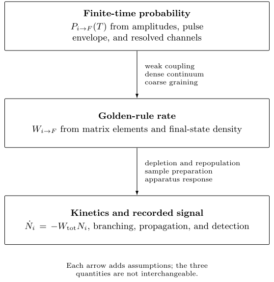
Three distinct description levels. A finite-time amplitude resolves pulse and observation windows. A golden-rule rate additionally assumes weak coupling, a sufficiently dense continuum, and coarse graining. Population kinetics and detector counts require depletion, branching, preparation, and apparatus models beyond the microscopic rate.

Validity window

A useful golden-rule window is schematically

$$\tau_{\mathrm{corr}} \ll T \ll \min \left( W^{-1}, t_{\mathrm{rec}} \right),$$

where:

• $\tau_{\mathrm{corr}}$ is the time over which the continuum or driving correlation loses memory;
• $W^{-1}$ is the depletion time;
• $t_{\mathrm{rec}}$ is a recurrence or discreteness time.

The left inequality permits energy coarse graining. The right inequalities keep first-order depletion small and prevent a finite spectrum from resolving into recurrences. The exact time scales depend on the model; this schematic inequality is a diagnostic, not a theorem with universal numerical factors.

The standard approximation also requires:

• weak coupling;
• a prepared initial state;
• a dense set of accessible final states;
• a matrix element and density of states that vary slowly over the finite-time energy window;
• negligible coherent return amplitude during the rate window;
• consistent normalization and degeneracy accounting.

Driven absorption and stimulated emission

For a harmonic perturbation, energy conservation includes the drive quantum. With the convention introduced above,

$$\begin{aligned} W_{i\rightarrow F}^{\mathrm{abs}} &= \frac{2\pi}{\hbar} \sum_{f\in F} \left| V_{fi}^{(+)} \right|^2 \\ &\quad\times \delta \left( E_f-E_i-\hbar\omega \right). \end{aligned}$$

The stimulated-emission contribution is

$$\begin{aligned} W_{i\rightarrow F}^{\mathrm{stim}} &= \frac{2\pi}{\hbar} \sum_{f\in F} \left| V_{fi}^{(-)} \right|^2 \\ &\quad\times \delta \left( E_f-E_i+\hbar\omega \right). \end{aligned}$$

Real pulses replace these ideal delta functions by their spectral envelopes. Strong coherent driving replaces constant-rate dynamics by Rabi oscillations, power broadening, and population redistribution.

Differential and total rates

When the detector resolves a continuum variable $\xi$, retain it:

$$\frac{dW}{d\xi} = \frac{2\pi}{\hbar} \left| M_{fi}(\xi) \right|^2 \rho(E_f,\xi) \delta(E_f-E_i).$$

The total accepted rate is

$$W_{\mathrm{acc}} = \int_{\mathrm{acceptance}} d\xi\, \frac{dW}{d\xi}.$$

Angular distributions, polarization correlations, and photoelectron spectra contain information that disappears in the total rate. Integrate only after deciding what the measurement resolves.

Density of Final States

State counting and units

The density per unit energy is

$$\rho_E(E) = \frac{dN}{dE}.$$

It has dimensions of inverse energy. If the continuum also carries channel labels $\alpha$,

$$\sum_f \longrightarrow \sum_\alpha \int dE\, \rho_\alpha(E).$$

The density must count each independent state once. Spin, polarization, magnetic sublevels, propagation directions, and identical-particle symmetry may already be included. Adding the same degeneracy again double counts the channel.

Coordinate changes

If $E=\hbar\omega$, then

$$\rho_\omega(\omega) = \frac{dN}{d\omega} = \hbar\rho_E(E).$$

Therefore,

$$\frac{2\pi}{\hbar} |V|^2\rho_E = \frac{2\pi}{\hbar^2} |V|^2\rho_\omega.$$

For ordinary frequency $E=h\nu$,

$$\rho_\nu(\nu) = h\rho_E(E).$$

The numerical density changes with the coordinate. A formula using $\rho_\omega$ cannot be inserted into a convention expecting $\rho_E$ without the Jacobian.

Example: a free particle in three dimensions

For a nonrelativistic free particle of mass $m$ in volume $\mathcal V$, with internal degeneracy $g$ and kinetic energy $E>0$,

$$\frac{\rho_E(E)}{\mathcal V} = \frac{g}{4\pi^2} \left( \frac{2m}{\hbar^2} \right)^{3/2} \sqrt E.$$

This square-root threshold factor enters photoionization and scattering problems when the remaining matrix element is smooth. Near a threshold, however, the matrix element, angular-momentum barrier, and long-range interaction can vary rapidly. Pulling them outside the finite-time integral may then fail.

Discrete states are not a continuum

For one isolated final state, the response is a finite-time transition probability or coherent oscillation, not a constant golden-rule rate. A quasi-continuum can support a rate only when many levels lie within the energy resolution $\hbar/T$ and recurrences occur later than the observation window.

Artificially broadening a sparse numerical spectrum can make a smooth plot, but it does not by itself establish a physical irreversible rate.

Density versus spectral function

In interacting systems, a bare density of eigenstates may not be the most useful object. The measured response can involve a spectral function or dynamical structure factor that already contains matrix elements, many-body continua, and finite lifetimes.

Do not multiply such a response function by an additional density of states unless its definition requires it. The relevant many-body conventions are developed in Spectral Functions and Lifetime and Spectral Weight.

Transition Rate Versus Probability

A dimensional dictionary

Quantity and symbol	Meaning and dimensions
Transition probability, $P_{i\to F}(T)$	Dimensionless fraction transferred by a specified time
Microscopic transition rate, $W_{i\to F}$	Events per prepared system per unit time; $\mathrm{s}^{-1}$
Spontaneous-emission coefficient, $A_{u\ell}$	Radiative decay rate for one channel; $\mathrm{s}^{-1}$
Cross section, $\sigma$	Rate divided by incident particle or photon flux; area
Event count rate, $R_{\mathrm{det}}$	Registered events per unit laboratory time; $\mathrm{s}^{-1}$
Energy width, $\Gamma_E$	Decay or response scale after a stated model; energy

The same word “transition probability” is sometimes used in atomic databases for an Einstein $A$ coefficient with units of $\mathrm{s}^{-1}$. Units reveal that this tabulated quantity is a rate, not a dimensionless Born probability.

Short-time, rate, and depletion regimes

Exact unitary dynamics begins quadratically at sufficiently short times:

$$P_{i\rightarrow F}(T) \propto T^2.$$

After continuum coarse graining, first-order perturbation theory gives a linear window:

$$P_{i\rightarrow F}(T) \approx W_{i\rightarrow F}T, \qquad WT\ll1.$$

This does not remain valid until $P>1$. Once depletion matters, a kinetic model may give

$$\frac{dN_i}{dt} = -W_{\mathrm{tot}}N_i,$$

with solution

$$N_i(t) = N_i(0)e^{-W_{\mathrm{tot}}t}.$$

The decay probability is then

$$P_{\mathrm{decay}}(t) = 1-e^{-W_{\mathrm{tot}}t}.$$

The exponential is a resummed, coarse-grained description. It is not the first-order result extrapolated blindly, and it does not reproduce the exact quadratic behavior arbitrarily close to $t=0$.

Hazard rate and nonexponential decay

For survival probability $S(t)$, define the instantaneous hazard

$$h(t) = - \frac{d}{dt} \ln S(t).$$

Exponential decay has constant $h(t)=W$. Structured reservoirs, coherent coupling, transport, trapping, and finite spectra can produce a time-dependent hazard. Quoting one lifetime for such dynamics requires a convention, such as an initial slope, a mean survival time, or a fitted model.

Competing channels, lifetime, and branching

For independent weak channels $c$,

$$W_{\mathrm{tot}} = \sum_c W_c, \qquad \tau = \frac{1}{W_{\mathrm{tot}}}.$$

The branching fraction is

$$b_c = \frac{W_c}{W_{\mathrm{tot}}}, \qquad \sum_c b_c=1.$$

The sum includes radiative and nonradiative channels if $\tau$ is the total population lifetime. A radiative rate alone predicts the measured lifetime only when quenching, predissociation, autoionization, collisions, and other losses are negligible.

Rate and linewidth

If an isolated upper-state amplitude evolves as

$$a_u(t) = \exp \left( -i\omega_u t -\frac{W_{\mathrm{tot}}t}{2} \right)$$

for $t\ge0$, its Fourier intensity is Lorentzian. With a stable lower state and no pure dephasing,

$$\Delta\omega_{\mathrm{FWHM}} = W_{\mathrm{tot}}, \qquad \Gamma_E = \hbar W_{\mathrm{tot}}.$$

Lower-state decay, pure dephasing, collisions, motion, unresolved structure, power broadening, and instrument response alter the observed width. The symbol $\Gamma$ is used in the literature for both a rate and an energy width; attach units or a subscript every time the distinction matters.

When a rate is the wrong language

Do not force a constant rate onto:

• a resonantly driven isolated two-level system showing Rabi oscillations;
• a Landau–Zener sweep through an avoided crossing;
• a short pulse whose bandwidth and phase are essential;
• coherent interference among several pathways;
• a sparse spectrum with observable recurrences;
• a strongly coupled system with dressed states;
• non-Markovian dynamics with memory;
• a measurement-conditioned quantum trajectory.

These problems have transition probabilities, amplitudes, response functions, or stochastic records, but not necessarily one time-independent rate.

Connection to Spectroscopy

From one-system rate to a sample signal

For $N_i$ independently prepared systems in an optically thin, weak-probe regime, a microscopic event rate gives

$$R_{\mathrm{events}} = N_i W_{i\rightarrow F}.$$

If the overall detection efficiency is $\eta$,

$$R_{\mathrm{det}} = \eta N_i W_{i\rightarrow F}.$$

This compact relation can fail through reabsorption, optical depth, state-dependent collection, detector dead time, saturation, spatial inhomogeneity, or population dynamics. A detector count rate is therefore not itself a molecular or atomic transition rate.

For optically thin spontaneous emission,

$$R_{\gamma,u\ell} = \eta N_u A_{u\ell},$$

while the emitted power contains an additional photon-energy factor:

$$P_{u\ell} = \hbar\omega_{u\ell} N_u A_{u\ell}.$$

Population and photon energy can change relative line intensities even when the $A$ coefficients are fixed.

Rate and cross section

For incident spectral photon flux $\Phi_\omega(\omega)$ and absorption cross section $\sigma(\omega)$,

$$W_{\mathrm{abs}} = \int_0^\infty d\omega\, \Phi_\omega(\omega) \sigma(\omega).$$

For a sufficiently narrow monochromatic probe,

$$W_{\mathrm{abs}} \approx \Phi\,\sigma.$$

Here $\Phi$ has dimensions of photons per area per time and $\sigma$ has dimensions of area. The relation holds per target in the weak, independent event regime. Propagation through a dense sample additionally requires radiative transfer or Maxwell–Bloch dynamics.

From an ideal delta function to a line profile

An ideal driven rate contains

$$\delta \left( E_f-E_i-\hbar\omega \right).$$

Finite coherence, motion, collisions, static disorder, and apparatus response replace this ideal constraint by a normalized profile. On an angular-frequency axis, one may write schematically

$$W_{i\rightarrow f}(\omega) = \mathcal W_{if} L_{if} \left( \omega-\omega_{fi} \right),$$

where

$$\int_{-\infty}^{\infty} L_{if}(\delta\omega)\, d\delta\omega = 1.$$

Then

$$\mathcal W_{if} = \int_{-\infty}^{\infty} W_{i\rightarrow f}(\omega)\, d\omega$$

is a frequency-integrated rate weight, with dimensions of rate times angular frequency. It is not generally a one-system rate by itself. Peak height is not invariant under broadening: a wider profile redistributes the same integrated weight.

The physical derivation of $L_{if}$ belongs to Line Shapes and Broadening. The chapter Spectroscopy overview gives the current Lorentzian, Gaussian, Voigt, $T_1$, and $T_2$ dictionary.

A calculation-to-measurement workflow

For a reproducible transition-rate prediction:

1. Declare the reference Hamiltonian. State which interactions define the eigenstates and which are treated as perturbations.
2. Specify preparation. Give populations, coherences, temperature, polarization, fields, and orientation.
3. Define the final channel. List resolved and summed quantum numbers, continuum coordinates, and detector acceptance.
4. Write the interaction. Include field normalization, polarization, envelope, multipole order, and gauge.
5. Evaluate matrix elements. State basis, normalization, angular averages, and convergence tests.
6. Choose finite-time or rate dynamics. Verify continuum, weak-coupling, smoothness, depletion, and recurrence conditions.
7. Count final states once. Document density-of-states units and every degeneracy factor.
8. Convert to the observable. Include populations, flux, branching, line profile, propagation, and detector response.
9. Propagate uncertainty. Separate numerical, structural, calibration, and model errors.

Comparing with tabulated data

Before comparing a calculated rate with a database value, verify:

• whether the entry is $A_{u\ell}$, $g_uA_{u\ell}$, oscillator strength, line strength, or a relative intensity;
• whether initial substates are averaged and final substates summed;
• the multipole type and any mixed-transition convention;
• wavelength, energy, and unit conventions;
• whether the value is measured, calculated, fitted, or inferred;
• uncertainty and bibliographic provenance.

The NIST Atomic Spectra Database, for example, distinguishes $A$ values, weighted $gA$ values, absorption oscillator strengths, line strengths, and relative intensities. Those columns are related, but they are not interchangeable labels for one number.

Common Mistakes

“The rate is the derivative of probability at zero time”

Exact unitary transition probability starts quadratically, so that derivative vanishes. A golden-rule rate is a coarse-grained intermediate-time slope after a continuum limit.

“The delta function is exact energy conservation at finite time”

A finite interaction produces a window of width of order $\hbar/T$. The delta function is a distributional long-time replacement under a smooth continuum integral.

“Final-state degeneracy should be averaged”

Accessible orthogonal final states are summed. An average over initial states appears only when the preparation assigns those populations.

“Different pathways always add as rates”

Pathways to the same indistinguishable final state add as amplitudes and can interfere.

“The density of states is just a number”

It depends on energy coordinate, volume convention, internal degeneracy, and which quantum numbers have already been integrated.

“A tabulated transition probability is dimensionless”

In atomic spectroscopy, that phrase often denotes an Einstein $A$ coefficient in $\mathrm{s}^{-1}$. Check units.

“A microscopic rate is a measured intensity”

Populations, photon energy, flux, propagation, collection, and detector response stand between them.

“A constant rate applies under strong resonant driving”

An isolated strongly driven transition is coherent and generally exhibits Rabi dynamics rather than irreversible golden-rule transfer.

Key Takeaways

• A transition channel must specify preparation, unresolved quantum numbers, continuum coordinates, and detector acceptance.
• Coherent pathways add as amplitudes; incoherent initial mixtures and orthogonal final records add as probabilities.
• Matrix elements and densities of states form one normalization-dependent product; arbitrary box factors must cancel.
• Fermi’s golden rule is a weak-coupling, continuum, coarse-grained limit of a finite-time probability.
• Probability is dimensionless, a rate has units of inverse time, a cross section has units of area, and a detector count rate includes sample and apparatus factors.
• Initial degeneracies are averaged only according to preparation; accessible final states are summed.
• Exponential decay and lifetime relations require a kinetic or open-system model beyond first-order probability.
• Spectroscopic comparison requires the precise meanings of $A$, $gA$, $f$, line strength, relative intensity, and linewidth to be kept distinct.

Exercises

Exercise 1: Normalize the finite-time kernel

Starting from

$$I_T(\Delta E) = \int_0^T dt\, e^{i\Delta E t/\hbar},$$

derive the expression for $K_T(\Delta E)$ used above and verify that $K_T(0)=T/(2\pi\hbar)$. Explain why its area remains one while its height grows with $T$.

Solution

For $\Delta E\ne0$,

$$\begin{aligned} I_T(\Delta E) &= \frac{\hbar} {i\Delta E} \left( e^{i\Delta E T/\hbar}-1 \right) \\ &= e^{i\Delta E T/(2\hbar)} \\ &\quad\times \frac{ 2\hbar \sin \left( \Delta E T/(2\hbar) \right) }{ \Delta E }. \end{aligned}$$

Therefore,

$$K_T(\Delta E) = \frac{2\hbar}{\pi T} \frac{ \sin^2 \left( \Delta E T/(2\hbar) \right) }{ (\Delta E)^2 }.$$

Taking the limit $\Delta E\to0$ and using $\sin x\sim x$ gives

$$K_T(0) = \frac{T}{2\pi\hbar}.$$

Parseval’s identity gives

$$\int_{-\infty}^{\infty} d(\Delta E)\, |I_T(\Delta E)|^2 = 2\pi\hbar T,$$

so the definition of $K_T$ makes its area one. Its height grows as $T$, while its central width shrinks as $\hbar/T$. The kernel approaches a delta distribution, not an ordinary function with a finite pointwise limit.

Exercise 2: Average and sum degeneracies

An unpolarized initial level has two equally populated substates $a=1,2$. A detector sums over three orthogonal final substates $b=1,2,3$. In common units, the squared matrix elements are

$$\left( |M_{ab}|^2 \right) = \begin{pmatrix} 1 & 4 & 0 \\ 2 & 1 & 2 \end{pmatrix}.$$

Assume the same density-of-states factor for every entry. Find the strength factor multiplying that common factor. What incorrect result follows from averaging over both initial and final states?

Solution

Sum over accepted final states and average over the equally populated initial states:

$$\begin{aligned} \overline{\mathcal S} &= \frac12 \sum_{a=1}^{2} \sum_{b=1}^{3} |M_{ab}|^2 \\ &= \frac12 \left[ (1+4+0) + (2+1+2) \right] \\ &= 5. \end{aligned}$$

Averaging over the three final states as well would give $5/3$. That would discard two thirds of the accepted orthogonal channels and would not represent the detector described in the question.

Exercise 3: Change the density coordinate

A calculation gives an energy density of states $\rho_E=3.0\times10^{18}\ \mathrm{J}^{-1}$. Find the corresponding density per angular frequency, $\rho_\omega$. Show that the golden-rule rate is unchanged when written in either convention.

Solution

Since $E=\hbar\omega$,

$$\rho_\omega = \hbar\rho_E.$$

Using $\hbar=1.054571817\times10^{-34}\ \mathrm{J\,s}$,

$$\begin{aligned} \rho_\omega &= 1.054571817\times10^{-34} \\ &\quad\times \left( 3.0\times10^{18} \right) \mathrm s \\ &\approx 3.16\times10^{-16}\ \mathrm s. \end{aligned}$$

The unit seconds is equivalent to states per $\mathrm{rad\,s^{-1}}$, with radians dimensionless. Because $\rho_E=\rho_\omega/\hbar$,

$$\frac{2\pi}{\hbar} |V|^2\rho_E = \frac{2\pi}{\hbar^2} |V|^2\rho_\omega.$$

The physical rate is unchanged; only the coordinate convention has changed.

Exercise 4: Lifetime and branching

An excited level has radiative rates

$$\begin{aligned} A_1 &= 2.0\times10^7\ \mathrm{s^{-1}}, \\ A_2 &= 3.0\times10^7\ \mathrm{s^{-1}}, \end{aligned}$$

and a nonradiative rate $W_{\mathrm{nr}}=5.0\times10^7\ \mathrm{s^{-1}}$. Find the total lifetime, the two radiative branching fractions, and the radiative quantum yield.

Solution

The total rate is

$$\begin{aligned} W_{\mathrm{tot}} &= A_1+A_2+W_{\mathrm{nr}} \\ &= 1.0\times10^8\ \mathrm{s^{-1}}. \end{aligned}$$

Therefore,

$$\tau = \frac{1}{W_{\mathrm{tot}}} = 10\ \mathrm{ns}.$$

The channel branching fractions are

$$\begin{aligned} b_1&=0.20, & b_2&=0.30, \\ b_{\mathrm{nr}}&=0.50. \end{aligned}$$

The radiative quantum yield is the sum of the radiative branches:

$$\Phi_{\mathrm{rad}} = \frac{A_1+A_2}{W_{\mathrm{tot}}} = 0.50.$$

Using only $A_1+A_2$ to infer the lifetime would predict $20\ \mathrm{ns}$ and would miss the nonradiative loss.

Exercise 5: From cross section to detector counts

A weak monochromatic beam has photon flux $\Phi=2.0\times10^{18}\ \mathrm{m^{-2}\,s^{-1}}$. The absorption cross section per target is $\sigma=3.0\times10^{-21}\ \mathrm{m^2}$. A sample contains $N=5.0\times10^7$ independent targets in the illuminated volume, and the event-detection efficiency is $\eta=0.12$. Estimate the single-target absorption rate and the detected count rate. State two assumptions behind the calculation.

Solution

The rate per target is

$$\begin{aligned} W_{\mathrm{abs}} &= \Phi\sigma \\ &= \left( 2.0\times10^{18} \right) \left( 3.0\times10^{-21} \right) \mathrm{s^{-1}} \\ &= 6.0\times10^{-3}\ \mathrm{s^{-1}}. \end{aligned}$$

The detected count rate is

$$\begin{aligned} R_{\mathrm{det}} &= \eta N W_{\mathrm{abs}} \\ &= (0.12) \left( 5.0\times10^7 \right) \\ &\quad\times \left( 6.0\times10^{-3}\ \mathrm{s^{-1}} \right) \\ &= 3.6\times10^4\ \mathrm{s^{-1}}. \end{aligned}$$

Assumptions include weak unsaturated absorption, negligible depletion, independent targets, uniform flux, negligible optical depth or reabsorption, and a rate-independent detection efficiency. At least two must be stated.

Exercise 6: Decide whether a rate applies

Compare two systems:

1. an isolated two-level atom driven resonantly by a coherent monochromatic field;
2. an unstable state weakly coupled to a broad continuum whose correlation time is much shorter than the observed decay time.

Which system naturally admits a constant transition rate, and what behavior is expected in the other?

Solution

The weakly coupled broad continuum naturally admits a golden-rule rate after coarse graining. Its survival can be approximately exponential over the Markovian window, subject to short-time and late-time corrections.

The isolated resonantly driven two-level atom has one discrete final state and retains phase coherence. It undergoes Rabi oscillations, with populations moving back and forth. A constant irreversible rate is not the natural description unless additional dephasing, ensemble averaging, or reservoir coupling destroys the coherence.

Exercise 7: Derive the length–velocity identity

For

$$\widehat H_0 = \frac{\widehat{\mathbf p}^{\,2}}{2m} + V(\widehat{\mathbf r}),$$

use the commutator $[\widehat H_0,\widehat{\mathbf r}]$ to show that exact energy eigenstates satisfy

$$\langle f|\widehat{\mathbf p}|i\rangle = i m\omega_{fi} \langle f|\widehat{\mathbf r}|i\rangle.$$

Why can approximate calculations violate this relation?

Solution

For a local potential,

$$\left[ \widehat H_0, \widehat{\mathbf r} \right] = - \frac{i\hbar}{m} \widehat{\mathbf p}.$$

Taking an energy-eigenstate matrix element gives

$$\begin{aligned} \langle f| [\widehat H_0,\widehat{\mathbf r}] |i\rangle &= (E_f-E_i) \langle f|\widehat{\mathbf r}|i\rangle \\ &= -\frac{i\hbar}{m} \langle f|\widehat{\mathbf p}|i\rangle. \end{aligned}$$

Solving for the momentum matrix element and using $E_f-E_i=\hbar\omega_{fi}$ yields

$$\langle f|\widehat{\mathbf p}|i\rangle = i m\omega_{fi} \langle f|\widehat{\mathbf r}|i\rangle.$$

A truncated basis or approximate state may not satisfy the eigenvalue equation and commutator identity accurately. Inconsistent effective Hamiltonians or omitted terms can also spoil equivalence between gauges.

Exercise 8: Audit a database comparison

A calculation reports a “transition probability” of $8.0\times10^6$ with no units and claims agreement with a database’s relative intensity of $7.5$. List the information needed before the comparison has physical meaning.

Solution

At minimum, determine:

1. whether the calculated number is a dimensionless finite-time probability, an $A$ coefficient, $gA$, an oscillator strength, or a line strength;
2. its units and normalization;
3. which initial substates were averaged and final substates summed;
4. the transition multipole and polarization convention;
5. the database column’s exact definition and units;
6. how the relative intensity depends on upper-state population, photon energy, plasma or source conditions, and detector response;
7. whether both values refer to the same isotope, charge state, levels, and environmental conditions;
8. uncertainties and bibliographic provenance.

A database relative intensity is generally not a direct measurement of one intrinsic matrix element. The two bare numbers cannot be compared as written.

Cross-Links

• Einstein Coefficient Reference gives the sharp-line rate, lifetime, branching, and detailed-balance ledger.
• Oscillator Strength Reference supplies the convention-explicit conversion and completeness checks for E1 strengths.
• Line Shape Reference converts decay and coherence rates into convention-explicit spectral widths.
• Spectroscopy
• Oscillator Strengths
• Einstein Coefficients
• Absorption and Emission
• Fluorescence and Phosphorescence
• Photoelectron Spectroscopy
• Line Shapes and Broadening
• Selection Rules in Spectroscopy
• Transition Probabilities
• First-Order Transition Probability
• Fermi’s Golden Rule
• Density of States in Transition Rates
• Selection Rules in Transition Rates
• Transition Rates in Light–Matter Interaction
• Resonant Driving
• Rabi Formula in the Weak-Drive Limit
• Atomic Selection Rules
• Molecular Symmetry
• Wigner–Eckart Theorem
• Quantum Optical Master Equation
• Optical Bloch Equations
• Spectral Functions

References

• P. A. M. Dirac, “The quantum theory of the emission and absorption of radiation,” Proceedings of the Royal Society A 114, 243–265 (1927), doi:10.1098/rspa.1927.0039.
• E. Fermi, Nuclear Physics: A Course Given by Enrico Fermi at the University of Chicago, University of Chicago Press, 1950; revised edition, 1974.
• V. Weisskopf and E. Wigner, “Berechnung der natürlichen Linienbreite auf Grund der Diracschen Lichttheorie,” Zeitschrift für Physik 63, 54–73 (1930), doi:10.1007/BF01336768.
• J. J. Sakurai and J. Napolitano, Modern Quantum Mechanics, 3rd ed., Cambridge University Press, 2020.
• C. Cohen-Tannoudji, B. Diu, and F. Laloë, Quantum Mechanics, Wiley, 1977.
• C. Cohen-Tannoudji, J. Dupont-Roc, and G. Grynberg, Atom–Photon Interactions: Basic Processes and Applications, Wiley, 1992.
• B. H. Bransden and C. J. Joachain, Physics of Atoms and Molecules, 2nd ed., Pearson, 2003.
• P. F. Bernath, Spectra of Atoms and Molecules, 5th ed., Oxford University Press, 2025, doi:10.1093/oso/9780197754498.001.0001.
• W. Demtröder, Laser Spectroscopy 1: Basic Principles, 5th ed., Springer, 2014, doi:10.1007/978-3-642-53859-9.
• A. Kramida, Yu. Ralchenko, J. Reader, and NIST ASD Team, NIST Atomic Spectra Database, Standard Reference Database 78, doi:10.18434/T4W30F.
• A. Kramida and J. R. Fuhr, NIST Atomic Transition Probability Bibliographic Database, Standard Reference Database 110, doi:10.18434/T46C7N.