Infrared Spectroscopy

Infrared spectroscopy measures how matter absorbs, emits, or reflects radiation in spectral regions where molecular rotations, vibrations, and low-lying electronic or collective excitations occur. In molecular vibrational spectroscopy, the leading coupling is usually electric dipole: an incident field drives a transition only when the molecular dipole operator has a nonzero matrix element between the initial and final states.

The practical inference chain is

$$\begin{gathered} \text{source and spectral encoder} \\ \downarrow \\ \text{sample-dependent radiant power} \\ \downarrow \\ \begin{matrix} \text{transmission, reflection,}\\ \text{or emission} \end{matrix} \\ \downarrow \\ \begin{matrix} \text{resolved lines or}\\ \text{vibrational bands} \end{matrix} \\ \downarrow \\ \begin{matrix} \text{molecular identity, abundance,}\\ \text{or structure} \end{matrix}. \end{gathered}$$

The first arrow is instrumental, the middle arrows require optical modeling, and the final arrow requires quantum assignments. A plotted “IR spectrum” therefore needs metadata: spectral coordinate, phase, temperature, pressure, sampling geometry, resolution, reference procedure, and intensity convention.

Canonical Scope

This page owns the infrared-specific workflow for:

• coupling an infrared electric field to a molecular dipole surface;
• converting dipole derivatives into harmonic-fundamental transition moments;
• applying vibrational, symmetry, polarization, and rotational selection rules;
• distinguishing transmission, Fourier-transform, attenuated-total-reflection, and reflectance measurements;
• recognizing rovibrational branch structure in gas-phase infrared bands;
• using characteristic-group and fingerprint regions without overclaiming molecular identification; and
• separating measured transmittance from intrinsic absorption strength.

Nearby pages supply the underlying pieces:

• Vibrational Spectroscopy
• Raman Spectroscopy owns harmonic and anharmonic term values, normal-mode assignments, overtones, combination bands, and force-field inference.
• Absorption and Emission owns Beer–Lambert propagation, cross sections, radiative transfer, and population effects for general spectroscopic transitions.
• Normal Modes of Polyatomics derives the mass-weighted Hessian and first-order infrared and Raman activity.
• Vibrational Spectra Computation computes anharmonic H$^{35}$Cl transition moments and compares relative overtone strengths with explicitly selected compiled band intensities.
• Selection Rules in Spectroscopy organizes exact, approximate, and operator-dependent selection rules.
• Rovibrational Coupling derives P, Q, and R branches, vibration-dependent rotational constants, and Coriolis structure.
• Spectroscopy as an Experimental Technique gives the broader instrument and evidence history.
• Terahertz and Infrared Probes in Quantum Matter develops complex electrodynamics, superconducting gaps and stiffness, crystal polar modes, and field-resolved THz measurements.

This page uses those results to answer an operational question: what does an infrared instrument record, and what can be inferred from it?

Infrared Coordinates and Windows

Wavenumber and wavelength

Mid-infrared molecular spectra are commonly plotted against vacuum wavenumber

$$\widetilde\nu = \frac{1}{\lambda_{\mathrm{vac}}},$$

usually in $\mathrm{cm}^{-1}$. Wavelength in micrometres is related by

$$\lambda_{\mathrm{vac}}(\mu\mathrm m) = \frac{10^4} {\widetilde\nu(\mathrm{cm}^{-1})}.$$

The photon energy is

$$E_\gamma = hc\widetilde\nu.$$

Many IR plots place high wavenumber at the left and let the axis decrease toward the right. That convention reverses the direction of a usual increasing-frequency graph. Always read the tick labels before interpreting “left” or “right.”

Near-, mid-, and far-infrared

The boundaries between infrared subregions are conventional rather than fundamental. A common laboratory partition is:

Region	Approximate wavenumber	Frequent molecular information
Near-infrared	$12{,}800$ to $4{,}000\ \mathrm{cm}^{-1}$	Overtone and combination bands, especially X–H motion
Mid-infrared	$4{,}000$ to $400\ \mathrm{cm}^{-1}$	Many molecular fundamentals and characteristic-group bands
Far-infrared	$400$ to roughly $10\ \mathrm{cm}^{-1}$	Low-frequency vibrations, torsions, intermolecular modes, lattice modes, and some rotations

Instrument sources, beam splitters, windows, detectors, and calibration methods change across these ranges. A quoted region boundary should therefore be treated as a working convention, not as a discontinuity in molecular physics.

Electric-Dipole Coupling

Long-wavelength interaction

If the field varies negligibly across a molecule, the leading interaction is

$$\hat H_{\mathrm{int}}(t) = -\hat{\boldsymbol\mu} \mathbin{\cdot} \mathbf E(t).$$

For a linearly polarized monochromatic component,

$$\mathbf E(t) = E_0\boldsymbol\epsilon\cos\omega t,$$

the transition amplitude contains

$$M_{fi} = \left\langle f\right| \boldsymbol\epsilon \mathbin{\cdot} \hat{\boldsymbol\mu} \left|i\right\rangle.$$

The resonance condition $E_f-E_i=\hbar\omega$ locates a possible transition; $M_{fi}$ determines whether the electric-dipole channel survives and how strongly it is driven. Frequency matching alone does not create absorption.

Magnetic-dipole, electric-quadrupole, vibronic, and collision-induced channels can matter when the electric-dipole term vanishes or exceptionally high sensitivity is available. Calling a band “forbidden” is always shorthand for a declared leading operator and symmetry limit.

Dipole surface and nuclear motion

Within a one-surface Born–Oppenheimer treatment, the electronic state defines a geometry-dependent molecular dipole surface

$$\boldsymbol\mu(\mathbf Q) = \left\langle \psi_{\mathrm{el}}(\mathbf Q) \right| \hat{\boldsymbol\mu} \left| \psi_{\mathrm{el}}(\mathbf Q) \right\rangle_{\mathrm{el}}.$$

The vibrational transition moment is then

$$\mathbf M_{v'v''} = \int \chi_{v'}^*(\mathbf Q) \boldsymbol\mu(\mathbf Q) \chi_{v''}(\mathbf Q) \,d\mathbf Q.$$

This expression separates two physical ingredients:

1. the nuclear wavefunctions and their overlap; and
2. the dipole surface generated by the electrons and nuclei.

A vibrational spectrum is therefore not determined by the potential-energy surface alone. Energies require the nuclear Hamiltonian; infrared intensities also require the dipole surface.

Dipole Moment Derivative

Linear expansion in normal coordinates

Near an equilibrium geometry, define the molecule-fixed dipole derivatives

$$\begin{aligned} \mu'_{a,k} &\equiv \left( \frac{\partial\mu_a} {\partial Q_k} \right)_e, \\ \mu''_{a,kl} &\equiv \left( \frac{\partial^2\mu_a} {\partial Q_k\partial Q_l} \right)_e. \end{aligned}$$

The local expansion is then

$$\begin{aligned} \mu_a(\mathbf Q) &= \mu_a^{(e)} +\sum_k\mu'_{a,k}Q_k \\ &\quad +\frac12\sum_{kl} \mu''_{a,kl}Q_kQ_l +\cdots. \end{aligned}$$

For a harmonic fundamental of mode $k$,

$$\left\langle1_k\right| Q_k \left|0_k\right\rangle = \sqrt{ \frac{\hbar} {2\Omega_k} }.$$

The leading transition-moment component is therefore

$$\begin{aligned} M_{a,k}^{10} &\approx \left( \frac{\partial\mu_a} {\partial Q_k} \right)_e \left\langle1_k\right| Q_k \left|0_k\right\rangle \\ &= \left( \frac{\partial\mu_a} {\partial Q_k} \right)_e \sqrt{ \frac{\hbar} {2\Omega_k} }. \end{aligned}$$

The mode is first-order infrared active if at least one component satisfies

$$\left( \frac{\partial\mu_a} {\partial Q_k} \right)_e \ne0.$$

The derivative’s numerical value depends on how $Q_k$ is normalized. A reported quantum-chemistry “IR intensity” also depends on program conventions and unit conversions. The physical transition moment is invariant only when the coordinate normalization, derivative, and oscillator matrix element are used consistently.

Permanent dipole versus dipole change

The equilibrium dipole $\boldsymbol\mu_e$ does not decide vibrational infrared activity.

• Carbon dioxide has no permanent dipole, yet its antisymmetric stretch and bend change the dipole and are infrared active.
• A polar molecule can have a normal mode whose dipole derivative vanishes by symmetry.

Pure rotational electric-dipole absorption and vibrational electric-dipole absorption therefore use related but different criteria: the former probes a permanent molecule-fixed dipole, while the latter probes a transition moment, whose leading harmonic term is a dipole derivative.

Isotropic and polarized samples

For a fixed molecular transition moment $\mathbf M$ and field polarization $\boldsymbol\epsilon$,

$$I \propto \left| \boldsymbol\epsilon \mathbin{\cdot} \mathbf M \right|^2.$$

An isotropic orientational average gives

$$\overline{ \left| \boldsymbol\epsilon \mathbin{\cdot} \mathbf M \right|^2 } = \frac13 \left|\mathbf M\right|^2.$$

In a single crystal, oriented film, molecular beam, or stretched polymer, that average is inappropriate. Polarization-dependent absorbance can reveal the direction of a transition dipole relative to a laboratory or crystal axis. The measured dichroism also depends on orientation distributions, Fresnel factors, and sampling geometry.

Infrared-Active Modes

Symmetry criterion

The general electric-dipole condition is

$$\Gamma(\psi_f) \otimes \Gamma(\mu_a) \otimes \Gamma(\psi_i) \supset \Gamma_{\mathrm{tot.sym.}}.$$

For a nondegenerate, totally symmetric vibrational ground state and a one-quantum fundamental, this reduces to

$$\Gamma(Q_k) \subset \Gamma(x,y,z).$$

The notation says that the mode must transform like at least one component of the dipole vector. It does not say that every non-totally-symmetric mode is active or that every totally symmetric mode is inactive. The answer depends on the point group and its vector representations.

Water and carbon dioxide

Water belongs to $C_{2v}$ at equilibrium. Its two $A_1$ modes and one $B_2$ mode transform like allowed dipole components, so all three fundamentals are infrared active.

Linear carbon dioxide has:

$$\begin{aligned} \nu_1 &: \Sigma_g^+ \quad\text{symmetric stretch},\\ \nu_2 &: \Pi_u \quad\text{doubly degenerate bend},\\ \nu_3 &: \Sigma_u^+ \quad\text{antisymmetric stretch}. \end{aligned}$$

The gerade symmetric stretch is electric-dipole inactive from the gerade ground state at leading order. The ungerade bend and antisymmetric stretch are active. Isotopic substitution, surfaces, solvents, crystals, anharmonic mixing, or higher-order processes can weaken the ideal symmetry classification without erasing its value as the starting point.

Allowed does not mean strong

Symmetry answers whether a matrix element is forced to zero. It does not set its magnitude. An allowed mode can be weak because

$$\left| \frac{\partial\boldsymbol\mu} {\partial Q_k} \right|$$

is small. Conversely, a nominally forbidden state can borrow intensity from a nearby bright state. Concentration, lower-state population, isotopic abundance, orientation, band overlap, and detector response further separate an intrinsic line strength from an observed peak height.

Selection-Rule Hierarchy

Harmonic vibrational rule

With harmonic states and only the dipole term linear in $Q_k$,

$$\Delta v_k=\pm1, \qquad \Delta v_{j\ne k}=0.$$

For absorption from a cold ground state, this selects fundamentals. The rule is approximate because a real potential and dipole surface contain higher orders.

The quadratic dipole term can connect harmonic states with

$$\Delta v_k=0,\pm2,$$

while anharmonic wavefunctions mix harmonic number states. These mechanisms produce overtone and combination intensity. Their band origins and resonance structure belong to Vibrational Spectroscopy.

Hot bands

A hot band starts in a thermally populated excited state. For a mode of wavenumber $\widetilde\nu_k$,

$$\frac{N_1}{N_0} \approx \exp\left( -\frac{hc\widetilde\nu_k} {k_{\mathrm B}T} \right)$$

before degeneracy and rotational factors are included. Low-frequency modes can therefore show appreciable hot-band structure at room temperature. Heating changes populations and line shapes; it does not alter the exact symmetry of an isolated equilibrium Hamiltonian.

Rotational and parity rules

In a gas, total angular momentum and parity add further conditions. A simple electric-dipole transition obeys the angular rule

$$\Delta J=0,\pm1,$$

with $J=0\leftrightarrow J=0$ excluded, but molecular projections, parity, electronic angular momentum, vibrational angular momentum, and nuclear-spin statistics decide which branches and subbranches actually exist.

The compact mnemonic must not be applied without the rest of the state labels. A diatomic $^1\Sigma\leftrightarrow{}^1\Sigma$ vibrational band has P and R branches but no Q branch; a degenerate bend of a linear polyatomic can have a strong Q branch.

Environment can relax molecular labels

In liquids and amorphous solids, free rotation is interrupted and rotational quantum numbers cease to organize resolved lines. In crystals, the site group or factor group may differ from the free-molecule point group. Surface selection rules can favor dipole components with particular orientations. Selection rules remain symmetry statements, but the relevant Hamiltonian and symmetry group have changed.

From Transition Moment to Measured Area

Line strength and profile

Write a molecular absorption cross section as

$$\sigma_{lu}(\widetilde\nu,T) = S_{lu}(T) g_{lu}(\widetilde\nu),$$

with normalized profile

$$\int g_{lu}(\widetilde\nu) \,d\widetilde\nu = 1.$$

Then

$$S_{lu}(T) = \int \sigma_{lu}(\widetilde\nu,T) \,d\widetilde\nu.$$

The integrated strength contains the transition moment, lower-state population, degeneracy, stimulated-emission correction, and the adopted spectral-coordinate convention. Peak height additionally depends on the line profile and instrument response. Two spectra can have the same integrated area and different maxima.

Column density and optical depth

For a uniform, nonemitting sample in a justified narrow-beam transmission model,

$$-\ln\mathcal T(\widetilde\nu) = \mathcal N_l \sigma_{lu}(\widetilde\nu),$$

where $\mathcal N_l$ is lower-state column density. Integration gives

$$\int -\ln\mathcal T(\widetilde\nu) \,d\widetilde\nu = \mathcal N_l S_{lu}.$$

Base-ten absorbance is

$$\mathcal A_{10} = -\log_{10}\mathcal T = \frac{-\ln\mathcal T}{\ln10}.$$

For a homogeneous solution under Beer–Lambert conditions,

$$\mathcal A_{10}(\widetilde\nu) = \varepsilon_{10}(\widetilde\nu)c\ell.$$

This relation is not automatic for an ATR spectrum, diffuse reflectance, strongly scattering powder, saturated band, chemically associating solution, or detector signal contaminated by emission. The general propagation derivation and its limits are canonical in Absorption and Emission.

What an FTIR Instrument Measures

Interferogram

A Fourier-transform infrared spectrometer commonly uses an interferometer to encode many spectral components into detector power as a function of optical path difference $\delta$. After subtracting the unmodulated component, an idealized even interferogram has the cosine-transform form

$$g(\delta) = \int_0^\infty \mathcal S(\widetilde\nu) \cos\left( 2\pi\widetilde\nu\delta \right) \,d\widetilde\nu.$$

The spectrum $\mathcal S(\widetilde\nu)$ is recovered by a Fourier transform, with phase correction and instrument-specific processing. A sample spectrum is usually ratioed to a background or reference spectrum to estimate transmittance or a related response.

The interferogram is not a spectrum with the horizontal axis relabeled. The Fourier transform, sampling grid, phase treatment, and instrument line shape are part of the measurement model.

Resolution and maximum path difference

If the interferogram is measured only to a maximum optical path difference $\delta_{\max}$, the nominal resolution scale is

$$\Delta\widetilde\nu \sim \frac{1}{\delta_{\max}},$$

up to the instrument’s chosen resolution criterion and apodization convention. Longer path difference provides finer spectral resolution. Zero-filling creates a denser plotted grid but does not add independent resolution.

Truncating an interferogram produces sidelobes in the instrument line shape. Apodization suppresses sidelobes at the cost of broadening the central response. The reported resolution should name the apodization and line-shape convention when nearby features or widths matter.

Background and atmospheric subtraction

The measured response includes source spectrum, beam-splitter throughput, optical windows, detector response, purge quality, and sample geometry. A background scan removes these factors only to the degree that they remain stable between measurements.

Water vapor and carbon dioxide in the beam path produce common narrow residuals when sample and background atmospheres differ. Temperature drift, source drift, changing purge, detector nonlinearity, and moving fringes can also survive ratioing. Removing a reproducible atmospheric line is a data processing step, not evidence that the sample lacks absorption there.

Sampling Geometries

Transmission

In transmission, the detector measures radiant power that passes through the sample and its windows. The method is conceptually closest to Beer–Lambert attenuation, but only after accounting for:

• reflection at interfaces;
• scattering and diffraction;
• absorption by windows, solvent, or matrix;
• nonuniform thickness or concentration;
• multiple internal reflections and interference fringes;
• detector dynamic range; and
• sample emission at elevated temperature.

A band with transmittance indistinguishable from zero is optically opaque under those conditions. Its clipped peak cannot yield a reliable integrated absorbance merely by taking a larger logarithm. A shorter path, lower concentration, isotopic dilution, or weaker band may be required.

Attenuated total reflection

In attenuated total reflection (ATR), light undergoes total internal reflection in a high-index internal-reflection element. An evanescent field samples material in contact with the interface.

For vacuum wavelength $\lambda_0$, crystal index $n_1$, sample index $n_2$, and incidence angle $\theta$ above the critical angle, define the field-amplitude penetration depth by

$$E(z) = E(0)e^{-z/d_p}.$$

For an ideal lossless two-medium interface,

$$d_p = \frac{\lambda_0} { 2\pi n_1 \sqrt{ \sin^2\theta - \left(n_2/n_1\right)^2 } }.$$

This $d_p$ is not automatically the effective Beer–Lambert path length. Absorption, anomalous dispersion, polarization, number of reflections, contact quality, and wavelength-dependent Fresnel factors all alter the ATR response. Because $d_p$ grows with wavelength, an uncorrected ATR spectrum can have intensity ratios different from a transmission spectrum.

ATR is surface-weighted rather than magically surface-exclusive. The sampled depth depends on optical constants and geometry, and poor contact can suppress or distort bands.

Reflectance and diffuse-reflectance methods

Specular reflectance measures an optical boundary-value problem. Peak shapes depend on both real and imaginary parts of the refractive index and can be derivative-like rather than absorption-like. Extracting optical constants may require Fresnel modeling and Kramers–Kronig-consistent analysis.

Diffuse reflectance from powders combines absorption and multiple scattering. Transforms such as Kubelka–Munk rely on assumptions about an optically thick, homogeneous, diffusely scattering medium. A transformed reflectance trace should not be labeled as transmission absorbance without its model.

Rovibrational Structure

One vibrational band, many rotational lines

An isolated gas-phase molecule usually rotates while it vibrates. A vibrational transition therefore generates a set of rotationally resolved lines. In the simplest linear-rotor approximation with the same rotational constant $\widetilde B$ in both vibrational states,

$$\begin{aligned} \widetilde\nu_P(J'') &\approx \widetilde\nu_0 -2\widetilde B J'', \\ \widetilde\nu_R(J'') &\approx \widetilde\nu_0 +2\widetilde B(J''+1). \end{aligned}$$

Here $P$ has $\Delta J=-1$, $R$ has $\Delta J=+1$, and $\widetilde\nu_0$ is the band origin. For a simple $^1\Sigma\leftrightarrow{}^1\Sigma$ diatomic band there is no Q branch at $\widetilde\nu_0$.

Real upper- and lower-state rotational constants differ, so line spacings are not exactly uniform. Centrifugal distortion, spin structure, isotope mixtures, Coriolis coupling, and resonances add further structure. Those derivations are developed in Rovibrational Coupling.

Band origin versus envelope maximum

The most intense point in a gas-phase band need not equal $\widetilde\nu_0$. Rotational populations and line-strength factors distribute area among branches, while finite resolution and broadening merge them into an envelope. A prominent Q branch can lie near the origin in some bands, but its presence is a symmetry and angular-momentum result, not a universal marker.

Reporting the envelope maximum as a vibrational frequency without the resolution, temperature, and branch model can introduce a systematic shift.

Condensed-phase bands

In liquids and amorphous solids, rotational fine structure is usually lost. Collisions, orientational disorder, site distributions, hydrogen bonding, and collective interactions broaden and shift the feature. In crystals, factor-group splitting, longitudinal–transverse optical splitting, and polarization selection can become important.

The absence of resolved P and R branches does not mean that molecular rotation was never part of the microscopic dynamics. It means the free-rotor quantum numbers no longer organize long-lived, spectrally resolved states.

Characteristic Groups and the Fingerprint Region

A useful but approximate partition

The mid-infrared spectrum is often divided near $1500\ \mathrm{cm}^{-1}$. Above that value, several local stretching motions fall into recognizable characteristic-group ranges. Between approximately $1500$ and $400\ \mathrm{cm}^{-1}$, bending, skeletal, and coupled motions often produce a denser pattern called the fingerprint region.

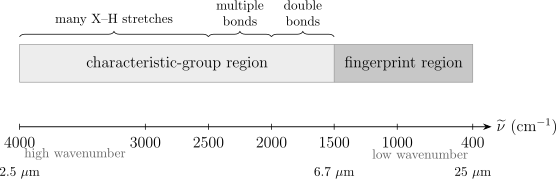
A conventional mid-infrared orientation, with wavenumber decreasing from left to right. The boundaries and group labels are assignment aids, not exact selection rules. The IUPAC fingerprint-region convention is often $1500$–$400\ \mathrm{cm}^{-1}$, and characteristic group frequencies can also occur inside it.

The phrase “fingerprint” should not be read too literally. The region is rich because many normal modes mix local stretches, bends, torsions, and skeletal coordinates. Similar molecules can have closely related patterns, while the same molecule can shift with phase, conformation, temperature, solvent, hydrogen bonding, crystal form, or isotope composition.

Characteristic frequencies are correlations

A correlation table is empirical structure–spectrum knowledge. It can suggest that a feature is compatible with a carbonyl, O–H, N–H, C–H, or other local motion. It does not replace a normal-mode calculation or a complete spectral assignment.

Band position depends on:

• local force constants and reduced-mass participation;
• conjugation, charge, and electronic structure;
• hydrogen bonding and coordination;
• vibrational coupling and resonance;
• conformer and phase;
• isotope substitution; and
• experimental calibration and sampling geometry.

Use ranges to generate hypotheses, then test those hypotheses against the whole spectrum and independent chemical information.

Library matching

A defensible library comparison should match, as closely as possible:

• chemical form, stereochemistry, and isotopic composition;
• gas, liquid, solution, matrix, amorphous, or crystalline phase;
• transmission, ATR, or reflectance geometry;
• spectral range and resolution;
• temperature and pressure;
• baseline and normalization method; and
• known contaminants or matrix bands.

Correlation or machine-learning similarity scores do not by themselves establish identity. Inspect which peaks drive the score, whether expected bands are absent, and whether mixtures or phase changes explain the residual.

Mixtures as an inverse problem

For a noninteracting homogeneous mixture under Beer–Lambert conditions,

$$\mathcal A_{10}^{\mathrm{mix}}(\widetilde\nu) = \ell \sum_j c_j \varepsilon_{10,j}(\widetilde\nu).$$

This linear model supports least-squares or constrained spectral unmixing. Identifiability fails when reference spectra are nearly collinear, the baseline is flexible enough to absorb real bands, strong components saturate, or chemical interactions change the component spectra. A small fit residual is not proof that the recovered concentrations are unique.

Practical Interpretation Workflow

1. Define the question. Identification, concentration, band assignment, orientation, kinetics, and optical constants require different measurements and models.
2. Record the sample. State composition, phase, thickness or path length, substrate or window, temperature, pressure, preparation, and time history.
3. Record the optical geometry. Distinguish transmission, ATR, specular reflection, diffuse reflection, and emission; include angle and polarization when relevant.
4. Acquire background and controls. Measure blank substrate, solvent, empty cell, purge atmosphere, or matrix as appropriate.
5. Preserve the raw interferogram or detector data. Document phase correction, apodization, zero-filling, atmospheric subtraction, smoothing, and baseline operations.
6. Check dynamic range. Flag clipped, saturated, negative-transmittance, or detector-nonlinear regions before fitting.
7. Assign from coarse to fine. Begin with phase and broad spectral families, then use symmetry, isotopes, polarization, temperature, and resolved structure.
8. Fit the measurement model. Convolve physical lines or bands with the instrument response and include baseline uncertainty rather than deconvolving blindly.
9. Validate externally. Predict withheld bands, concentrations, isotope shifts, temperatures, or independent measurements.
10. Report layers of inference. Separate raw response, processed spectrum, peak parameters, quantum assignment, and chemical conclusion.

Common Artifacts and Mistakes

Problem	Spectral symptom	Diagnostic or remedy
Atmospheric water or carbon dioxide mismatch	Narrow positive and negative residuals at familiar gas lines	Improve purge and compare sample and background timing
Interference fringes	Approximately periodic oscillation in wavenumber	Change thickness or angle and model multiple reflections
Scattering from particles or rough surfaces	Sloping or curved baseline, distorted strong bands	Change particle size or geometry and use a scattering-aware model
ATR contact variation	Irreproducible intensities with similar positions	Control pressure, contact area, crystal cleanliness, and sample surface
Optical saturation	Flat-bottomed or clipped strong bands	Shorten path or reduce concentration; do not fit the clipped core
Detector or source changeover	Step or response discontinuity	Inspect instrument channels and reference procedure
Overaggressive baseline subtraction	Negative lobes or removed broad bands	Fit controls and propagate baseline uncertainty
Unresolved gas rotational structure	Envelope maximum mistaken for band origin	Increase resolution or fit a rovibrational model

Calling transmittance loss pure absorption

Total transmittance can fall because of reflection, scattering, diffraction, or collection geometry. Use “absorbance” quantitatively only when the measurement model isolates absorption, or explicitly state that the plotted quantity also contains nonabsorptive attenuation.

Comparing ATR and transmission peak heights directly

ATR has wavelength-, polarization-, contact-, and index-dependent sampling. Relative heights can differ even for the same material. Compare corrected responses or use a library measured in the same geometry.

Reading one characteristic peak as an identification

A single band usually has many plausible carriers. Require a coherent pattern, absence of contradictory bands, proper phase matching, and independent sample context.

Treating zero-filling as higher resolution

Zero-filling interpolates the Fourier-transformed grid. It can make plots and peak localization smoother, but the measured maximum path difference and instrument line shape still determine independent resolution.

Equating a computed harmonic mode with an observed peak

The calculation may omit anharmonicity, environment, rotational structure, resonance, and electronic-structure error. State whether a scale factor or anharmonic correction was used and compare like quantities.

Key Takeaways

• Infrared vibrational absorption is controlled by a transition dipole, whose leading harmonic term is a dipole derivative along a normal coordinate.
• A permanent molecular dipole is neither necessary nor sufficient for a particular vibrational fundamental.
• Symmetry determines zeros; derivative magnitude, population, orientation, line shape, abundance, and instrument response determine observed strength.
• FTIR records an interferogram and reconstructs a spectrum; maximum optical path difference, apodization, and phase processing belong to the resolution statement.
• Transmission, ATR, and reflectance are different optical boundary-value problems and should not be compared as though they share one path length.
• Gas-phase vibrational bands can contain resolved P, Q, and R structure; condensed phases generally produce shifted and broadened bands.
• The fingerprint region supports identification through whole-pattern comparison, not by guaranteeing uniqueness from one peak.

Exercises

Exercise 1: Convert a carbonyl-region band

An absorption maximum occurs at $1715\ \mathrm{cm}^{-1}$. Find its vacuum wavelength in micrometres and photon energy in electronvolts. Use $hc=1.23984198\times10^{-4}\ \mathrm{eV\,cm}$.

Solution

The wavelength is

$$\begin{aligned} \lambda(\mu\mathrm m) &= \frac{10^4}{1715} \\ &\approx 5.831\ \mu\mathrm m. \end{aligned}$$

The photon energy is

$$\begin{aligned} E_\gamma &= \left( 1.23984198\times10^{-4} \right)(1715) \\ &\approx 0.2126\ \mathrm{eV}. \end{aligned}$$

The energy is much smaller than a typical visible photon energy but matches a molecular vibrational scale.

Exercise 2: Fundamental transition moment

For one mass-weighted harmonic mode,

$$\mu_x(Q) = \mu_e+aQ,$$

with all other dipole components independent of $Q$. Find the leading $1\leftarrow0$ transition moment and its isotropic polarization average.

Solution

The constant term cannot connect orthogonal harmonic states. Therefore

$$\begin{aligned} M_x^{10} &= a\langle1|Q|0\rangle \\ &= a \sqrt{ \frac{\hbar}{2\Omega} }. \end{aligned}$$

The molecular transition moment lies along $x$, so

$$\left|\mathbf M^{10}\right|^2 = |a|^2 \frac{\hbar}{2\Omega}.$$

For an isotropic ensemble and one fixed linear polarization,

$$\overline{ \left| \boldsymbol\epsilon \mathbin{\cdot} \mathbf M^{10} \right|^2 } = \frac13 |a|^2 \frac{\hbar}{2\Omega}.$$

The result assumes the stated mass-weighted coordinate convention.

Exercise 3: Carbon dioxide activity

Carbon dioxide has a gerade vibrational ground state. Use inversion parity to classify the leading electric-dipole infrared activity of its $\Sigma_g^+$ symmetric stretch, $\Pi_u$ bend, and $\Sigma_u^+$ antisymmetric stretch.

Solution

The electric dipole is ungerade. Starting from a gerade ground state, the triple product

$$\Gamma_f \otimes \Gamma(\boldsymbol\mu) \otimes \Gamma_i$$

can be gerade only when the final vibrational state is ungerade. The $\Pi_u$ bend and $\Sigma_u^+$ antisymmetric stretch can therefore be infrared active. The $\Sigma_g^+$ symmetric stretch is inactive at leading electric-dipole order.

Parity is necessary but the complete vector-representation condition is still required in a general point group.

Exercise 4: Overtone mechanism

Suppose the vibrational potential is harmonic but

$$\mu(Q) = \mu_e+aQ+bQ^2.$$

Which term can drive $2\leftarrow0$? Would the answer change if the dipole were strictly linear but the potential were anharmonic?

Solution

For harmonic states,

$$\langle2|Q|0\rangle=0, \qquad \langle2|Q^2|0\rangle\ne0.$$

The quadratic dipole term $bQ^2$ therefore drives the overtone through electrical anharmonicity.

If the dipole is linear but the potential is anharmonic, the exact wavefunctions mix harmonic number states. Then the matrix element of $Q$ between the exact ground and overtone states can be nonzero. That is mechanical anharmonicity. Real overtone intensity can contain both effects.

Exercise 5: Transmission and absorbance

A sample has measured transmittance $\mathcal T=0.250$ at one wavenumber. Find its decadic absorbance and Napierian optical depth. If Beer–Lambert conditions hold with $c=2.00\times10^{-3}\ \mathrm{mol\,L^{-1}}$ and $\ell=0.100\ \mathrm{cm}$, find the molar decadic absorption coefficient.

Solution

The decadic absorbance is

$$\begin{aligned} \mathcal A_{10} &= -\log_{10}(0.250) \\ &= 0.60206. \end{aligned}$$

The optical depth is

$$\begin{aligned} \tau &= -\ln(0.250) \\ &= 1.38629. \end{aligned}$$

Finally,

$$\begin{aligned} \varepsilon_{10} &= \frac{\mathcal A_{10}}{c\ell} \\ &= \frac{0.60206} {(2.00\times10^{-3})(0.100)} \\ &\approx 3.01\times10^3\ \mathrm{L\,mol^{-1}\,cm^{-1}}. \end{aligned}$$

The numerical result is meaningful only if reflection, scattering, concentration chemistry, and detector nonlinearity are negligible or corrected.

Exercise 6: FTIR path difference

An FTIR scan reaches a maximum optical path difference of $2.0\ \mathrm{cm}$. Estimate its nominal wavenumber-resolution scale. What happens if the interferogram is zero-filled to four times as many points?

Solution

The scale is

$$\Delta\widetilde\nu \sim \frac{1}{2.0\ \mathrm{cm}} = 0.50\ \mathrm{cm}^{-1}.$$

The exact quoted resolution depends on apodization and the instrument’s criterion. Fourfold zero-filling makes the transformed sampling grid four times denser, but it does not narrow the instrument line shape or add independent information. The physical resolution remains set by the measured path range.

Exercise 7: ATR penetration depth

For an ATR measurement at $\lambda_0=10.0\ \mu\mathrm m$, take $n_1=2.40$, $n_2=1.50$, and $\theta=45.0^\circ$. Verify total internal reflection and calculate the field-amplitude penetration depth.

Solution

The critical angle satisfies

$$\sin\theta_c = \frac{n_2}{n_1} = 0.625,$$

so

$$\theta_c\approx38.7^\circ.$$

Because $45.0^\circ>\theta_c$, total internal reflection occurs. The penetration depth is

$$\begin{aligned} d_p &= \frac{10.0\ \mu\mathrm m} {2\pi(2.40)} \\ &\quad\times \left[ \sin^2 45^\circ - \left(\frac{1.50}{2.40}\right)^2 \right]^{-1/2} \\ &\approx 2.01\ \mu\mathrm m. \end{aligned}$$

This is the $1/e$ field-amplitude scale under the ideal interface model, not a universal transmission-equivalent path length.

Exercise 8: A suspicious library match

An ATR spectrum of an unknown polymer gives a high library score for a reference measured in transmission. The strongest fingerprint peaks align, but their relative heights differ and a broad O–H feature is present only in the unknown. Give at least five checks before declaring an identification.

Solution

Useful checks include:

1. compare with an ATR reference or apply a justified ATR correction;
2. inspect contact pressure, crystal cleanliness, and sample surface;
3. test whether the O–H band is water, surface oxidation, additive, or a real polymer functional group;
4. compare the full spectrum, including expected weak bands and absent bands;
5. match phase, crystallinity, temperature, and polymer orientation;
6. inspect baseline, atmospheric subtraction, saturation, and resolution;
7. test plausible mixtures, fillers, plasticizers, and copolymers; and
8. confirm with an independent method or a second sampling geometry.

A high similarity score is evidence for a candidate, not a proof of unique identity. Geometry-dependent intensity and an unexplained broad band are specific reasons to withhold the stronger claim.

Cross-Links

• Spectroscopy Nomenclature fixes reciprocal-centimetre, absorbance, optical-depth, linewidth, and rovibrational branch conventions used in infrared spectra.
• Spectroscopy
• Vibrational Spectroscopy
• Absorption and Emission
• Transition Rates
• Line Shapes and Broadening
• Selection Rules in Spectroscopy
• Rotational Spectroscopy
• Vibrations of Diatomics
• Normal Modes of Polyatomics
• Rovibrational Coupling
• Molecular Symmetry
• Dipole Transitions
• Selection Rules and Transition Rates
• Spectroscopy as an Experimental Technique

References

• E. B. Wilson Jr., J. C. Decius, and P. C. Cross, Molecular Vibrations: The Theory of Infrared and Raman Vibrational Spectra, McGraw–Hill, 1955; Dover reprint, 1980.
• G. Herzberg, Molecular Spectra and Molecular Structure. II. Infrared and Raman Spectra of Polyatomic Molecules, Van Nostrand, 1945.
• P. F. Bernath, Spectra of Atoms and Molecules, 5th ed., Oxford University Press, 2025, doi:10.1093/oso/9780197754498.001.0001.
• P. R. Griffiths and J. A. de Haseth, Fourier Transform Infrared Spectrometry, 2nd ed., Wiley, 2007, doi:10.1002/047010631X.
• N. J. Harrick, Internal Reflection Spectroscopy, Interscience, 1967.
• M. Milosevic, Internal Reflection and ATR Spectroscopy, Wiley, 2012.
• Z. Movasaghi, S. Rehman, and I. U. Rehman, “Fourier Transform Infrared Spectroscopy of Biological Tissues,” Applied Spectroscopy Reviews 43, 134–179 (2008), doi:10.1080/05704920701829043.
• International Union of Pure and Applied Chemistry, “fingerprint region”, Compendium of Chemical Terminology, 5th ed., online version 5.0.0, 2025, doi:10.1351/goldbook.08604.
• H. Goenaga Infante et al., “Glossary of Methods and Terms Used in Analytical Spectroscopy,” Pure and Applied Chemistry 93, 647–776 (2021), doi:10.1515/pac-2019-0203.
• International Union of Pure and Applied Chemistry, “transmittance” and “Beer–Lambert law”, Compendium of Chemical Terminology, accessed 2026-07-22.
• NIST Chemistry WebBook, SRD 69, Carbon dioxide gas-phase infrared spectrum, accessed 2026-07-22.
• NIST Sensor Science Division, Fourier Transform Infrared Spectrophotometry Facility, accessed 2026-07-22.
• HITRANonline, Line-by-Line Definitions and Units and Cross-Section Definitions, accessed 2026-07-22.