Vibrational Spectra Computation

A computed vibrational spectrum is not one eigenvalue calculation. It is a chain connecting a potential-energy surface, nuclear masses, a finite representation, vibrational eigenstates, a transition-property surface, and the observable reported by an experiment. A frequency calculation can be numerically converged while the potential is inaccurate. Accurate energies do not imply accurate intensities. A list of vibrational term values is not yet an infrared or Raman spectrum.

This notebook makes those distinctions concrete with two deliberately small benchmarks:

1. a mass-weighted, stretch-only Hessian for linear $^{12}$C$^{16}$O$_2$, calibrated to declared harmonic target frequencies;
2. a one-dimensional Morse model for H$^{35}$Cl, parameterized from spectroscopic constants and solved by sinc discrete variable representation (DVR).

The first calculation exposes normal-mode projection, a translational zero mode, inversion parity, and the difference between infrared and Raman activity. The second separates harmonic error, anharmonic model error, discretization error, transition-property error, and comparison with compiled spectroscopic data.

The retained results are:

Quantity	Computed value	What it establishes
CO$_2$ symmetric stretch	$1354.000000000\ \mathrm{cm}^{-1}$	calibrated Hessian target recovered
CO$_2$ antisymmetric stretch	$2396.000000000\ \mathrm{cm}^{-1}$	calibrated Hessian target recovered
H$^{35}$Cl Morse dissociation parameter	$42341.901193347\ \mathrm{cm}^{-1}$	value implied by $\omega_e$ and $\omega_ex_e$
H$^{35}$Cl DVR fundamental	$2885.309100000\ \mathrm{cm}^{-1}$	numerical Morse term difference
H$^{35}$Cl higher-order term difference	$2885.977402500\ \mathrm{cm}^{-1}$	value implied by selected compiled constants
largest DVR error for $v=0,\ldots,7$	$3.64\times10^{-11}\ \mathrm{cm}^{-1}$	solver verified against exact Morse levels

The tiny DVR error verifies the implementation for the Morse Hamiltonian. It does not show that the Morse model predicts HCl spectroscopy to eleven decimal places. The $0.6683\ \mathrm{cm}^{-1}$ difference between the Morse and higher-order term values is already about ten orders of magnitude larger than the numerical error.

Run the investigation. The program and retained results below support the stated experiment. Follow Running an Experiment for environment and output-directory guidance. The recorded evidence applies to its stated parameters and environment.

Purpose and Canonical Scope

This page is the canonical home for the executable calculation that:

• constructs and diagonalizes a mass-weighted molecular Hessian;
• detects rigid translation and validates normal-mode normalization;
• assigns inversion parity and leading IR/Raman activity in a transparent CO$_2$ stretch model;
• constructs a Morse potential from H$^{35}$Cl spectroscopic constants;
• diagonalizes a one-dimensional vibrational Hamiltonian with sinc DVR;
• verifies numerical levels against the exact Morse spectrum;
• evaluates vibrational transition moments from a local dipole surface;
• compares band origins and relative intensities with compiled data; and
• reports a layered error and reproducibility record.

Neighboring pages retain broader canonical responsibilities:

• Normal Modes of Polyatomics owns the full Cartesian and internal-coordinate normal-mode theory, translation and rotation projection, molecular symmetry, degeneracy, Wilson’s $GF$ method, and production frequency-analysis workflow.
• Vibrations of Diatomics owns the physical reduction to a radial nuclear coordinate and the rovibrational interpretation of diatomic states.
• Vibrational Spectroscopy owns band assignments, anharmonic spectral structure, hot bands, overtones, combination bands, and force-field inference.
• Infrared Spectroscopy owns electric-dipole absorption, instrument response, and IR data interpretation.
• Raman Spectroscopy owns polarizability tensors, Raman selection rules, polarization observables, and Raman instrumentation.
• Potential-Energy Surfaces owns the electronic-structure origin, topology, and dimensionality of molecular potentials.
• Numerical Mathematics owns the general theory of finite representations, eigensolvers, convergence studies, conditioning, and floating-point error.

The present page therefore uses a small Hessian and a one-dimensional DVR as auditable computational examples. It does not duplicate a general normal-mode course or treat a stick list as a complete laboratory spectrum.

Reproducibility Contract

The executable artifact is a NumPy-only Python program:

• Download the program
• CO$_2$ normal-mode data
• H$^{35}$Cl potential data
• H$^{35}$Cl level data
• H$^{35}$Cl transition data
• H$^{35}$Cl convergence data
• Machine-readable metadata and validation

Run the downloaded program from the folder where you saved it:

python vibrational-spectra.py --output-dir results

The default run uses:

Item	Declared choice
language	Python 3
numerical dependency	NumPy
random numbers	none
internal units	atomic units
H$^{35}$Cl coordinate	$q=R-R_e$
DVR interval	$-1.5\le q/a_0\le12$
DVR points	$201$
DVR spacing	$0.0675a_0$
retained level comparison	$v=0,\ldots,9$
retained transitions	$v=0\to1,\ldots,5$
matrix eigensolver	real-symmetric numpy.linalg.eigh

The program contains no hidden optimization, stochastic seed, fitted correction after diagonalization, or external quantum-chemistry call. Its metadata records the runtime versions, constants, model parameters, matrices, grid, validation thresholds, source identifiers, and limitations.

The two claims are intentionally different

The CO$_2$ calculation is a calibrated algebra benchmark. Its two force constants are chosen to reproduce two declared stretch frequencies. Recovery of those frequencies validates matrix assembly and mode assignment, not the quality of an electronic-structure force field.

The H$^{35}$Cl calculation is a representation and model-hierarchy benchmark. The two Morse parameters are inferred from $\omega_e$ and $\omega_ex_e$. Agreement with the two-term Morse formula verifies the DVR. Comparison with $\omega_ey_e$, $\omega_ez_e$, and measured band intensities then reveals physics omitted by that fitted model.

Calling either calculation an independent first-principles prediction would erase the most important fact about its provenance.

From a Potential to a Spectrum

A useful computational dependency graph is

$$\begin{gathered} V(\mathbf R),\quad \{M_A\} \longrightarrow K,\ F \longrightarrow \{\omega_k,\mathbf e_k\} \\ \longrightarrow H_{\mathrm{vib}} \longrightarrow \{E_v,\chi_v\} \\ \mu(\mathbf Q),\ \boldsymbol\alpha(\mathbf Q) \longrightarrow \{\tilde\nu_{fi},S_{fi}\} \longrightarrow \text{experiment-facing spectrum}. \end{gathered}$$

Each arrow introduces distinct assumptions:

Layer	Representative input	Representative failure
electronic model	Born–Oppenheimer surface $V(\mathbf R)$	correlation, relativistic, or basis error
nuclear model	isotope masses, dimensionality	omitted rotation, coupling, nonadiabaticity
local approximation	Hessian at one minimum	anharmonicity, multiple minima, resonance
representation	basis or coordinate grid	truncation or boundary error
solver	symmetric diagonalization	residual or orthogonality failure
transition surface	$\mu(\mathbf Q)$ or $\boldsymbol\alpha(\mathbf Q)$	wrong derivatives or limited expansion
observation model	populations and line profiles	wrong temperature, pressure, or instrument response

This hierarchy matters because an energy residual tests only the solver layer. A measured intensity can be much more sensitive to the transition surface than the corresponding band origin is to the potential.

Harmonic Approximation

Let $\mathbf u$ collect Cartesian nuclear displacements from a stationary geometry $\mathbf R_e$. Expanding the potential gives

$$V(\mathbf R_e+\mathbf u) = V(\mathbf R_e) + \frac12 \mathbf u^{\mathsf T}K\mathbf u + O(\|\mathbf u\|^3),$$

where

$$K_{A\alpha,B\beta} = \left. \frac{\partial^2V} {\partial R_{A\alpha}\partial R_{B\beta}} \right|_{\mathbf R_e}.$$

The linear term vanishes only if the geometry is stationary to the relevant accuracy. The Cartesian equation of motion is

$$M\ddot{\mathbf u}+K\mathbf u=0,$$

with diagonal mass matrix $M$. The generalized eigenproblem is

$$K\mathbf l_k = \omega_k^2M\mathbf l_k.$$

Mass weighting converts it to an ordinary symmetric problem:

$$\begin{aligned} F &= M^{-1/2}KM^{-1/2}, \\ F\mathbf e_k &= \omega_k^2\mathbf e_k, \\ \mathbf l_k &= M^{-1/2}\mathbf e_k. \end{aligned}$$

If the mass-weighted eigenvectors satisfy $\mathbf e_j^{\mathsf T}\mathbf e_k=\delta_{jk}$, then the Cartesian vectors satisfy

$$\mathbf l_j^{\mathsf T}M\mathbf l_k = \delta_{jk}.$$

The spectroscopic harmonic wavenumber is

$$\tilde\nu_k = \frac{\omega_k}{2\pi c} = \frac{\hbar\omega_k}{hc}.$$

In atomic units, $\hbar=1$, so the program converts an angular frequency to wavenumber by multiplying by $219474.63136320\ \mathrm{cm}^{-1}$ per hartree.

What harmonic does and does not mean

The harmonic approximation is local in configuration space. It assumes:

• one stable equilibrium;
• a quadratic potential over the wavefunction’s relevant support;
• constant masses and a chosen coordinate metric;
• separable normal coordinates after the quadratic transformation; and
• transition-property expansions that may be truncated independently.

It does not imply that chemical bonds are literal springs over arbitrary displacements. It does not provide dissociation. It cannot produce intrinsic anharmonic overtones from a linear dipole surface. It also cannot describe Fermi resonance, large-amplitude torsion, tunneling between minima, or a conical-intersection region.

CO₂ Stretch-Only Hessian

The first benchmark retains only collinear displacements

$$\mathbf u = \begin{pmatrix} u_L & u_C & u_R \end{pmatrix}^{\mathsf T}$$

for O$_L$–C–O$_R$. Define the two bond extensions

$$\delta r_1=u_C-u_L, \qquad \delta r_2=u_R-u_C.$$

The declared model potential is

$$V_{\mathrm{str}} = \frac{k_b}{2} \left( \delta r_1^2+\delta r_2^2 \right) + \frac{k_{13}}{2} \left( \delta r_1+\delta r_2 \right)^2.$$

Equivalently,

$$K = k_b \begin{pmatrix} 1 & -1 & 0\\ -1 & 2 & -1\\ 0 & -1 & 1 \end{pmatrix} + k_{13} \begin{pmatrix} 1 & 0 & -1\\ 0 & 0 & 0\\ -1 & 0 & 1 \end{pmatrix}.$$

Every row sums to zero. Therefore uniform translation $\mathbf u\propto(1,1,1)^{\mathsf T}$ is an exact null vector before any diagonalization.

For $m_L=m_R=m_O$, the two stretch frequencies have closed forms:

$$\begin{aligned} \omega_s^2 &= \frac{k_b+2k_{13}}{m_O}, \\ \omega_a^2 &= k_b \left( \frac{1}{m_O}+\frac{2}{m_C} \right). \end{aligned}$$

The program solves these relations backward for a pedagogical force field whose declared targets are

$$\tilde\nu_s=1354\ \mathrm{cm}^{-1}, \qquad \tilde\nu_a=2396\ \mathrm{cm}^{-1}.$$

Using $^{12}$C and $^{16}$O isotopic masses gives

$$\begin{aligned} k_b &= 0.947\,929\,347\,135\,246 \frac{E_{\mathrm h}}{a_0^2}, \\ k_{13} &= 0.080\,891\,860\,307\,196 \frac{E_{\mathrm h}}{a_0^2}. \end{aligned}$$

These are fitted model parameters, not reported experimental C–O force constants and not the output of an electronic-structure calculation.

Numerical modes

The diagonalization returns:

Mode	$\tilde\nu$ ($\mathrm{cm}^{-1}$)	Relative $(u_L,u_C,u_R)$	Inversion	Leading activity
translation	$0$	$(1,1,1)$	ungerade	not a vibration
symmetric stretch	$1354.000000000$	$(-1,0,1)$	gerade	Raman allowed, IR forbidden
antisymmetric stretch	$2396.000000000$	$(0.375119,-1,0.375119)$	ungerade	IR allowed, Raman forbidden

For the antisymmetric stretch, centre-of-mass stationarity requires

$$2m_Ou_O+m_Cu_C=0,$$

so choosing $u_C=-1$ gives

$$u_O = \frac{m_C}{2m_O} = 0.375119\ldots.$$

The unequal Cartesian amplitudes are a mass effect. Plotting only arrows of equal length would obscure the normal coordinate actually diagonalized.

Validation of the Hessian calculation

The retained tests are:

Check	Measured diagnostic	Threshold
translational invariance	$\max_i\lvert\sum_jK_{ij}\rvert=0$	$10^{-14}E_{\mathrm h}/a_0^2$
symmetry of $F$	$0$	$10^{-14}$
eigenvector orthonormality	$4.82\times10^{-16}$	$10^{-12}$
analytic frequency agreement	$9.09\times10^{-13}\ \mathrm{cm}^{-1}$	$10^{-7}\ \mathrm{cm}^{-1}$
vibrational centre-of-mass residual	$1.42\times10^{-13}$	$10^{-10}$
inversion-parity error	$2.22\times10^{-16}$	$10^{-12}$

The numerical eigensolver represents the translational eigenvalue by a tiny roundoff-scale number. The program sets eigenvalues below $10^{-14}$ times the largest eigenvalue to zero. This is not used as the translation test: the exact Hessian row sums provide that independent check.

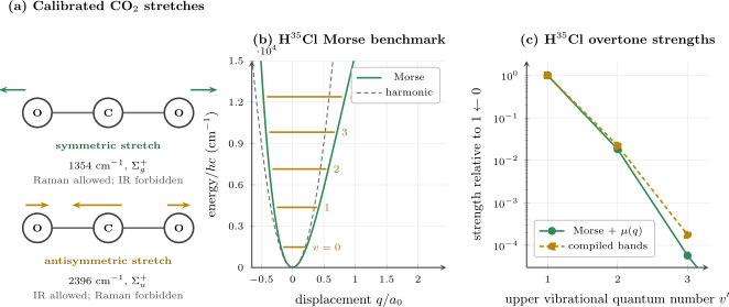
Two distinct benchmarks. Panel (a) shows the calibrated CO$_2$ stretch patterns and their leading centrosymmetric IR/Raman activity. Panel (b) compares the H$^{35}$Cl harmonic and Morse potentials with the first five DVR levels. Panel (c) compares relative $v=0\to v'$ intensity proxies from the Morse wavefunctions and local dipole polynomial with selected compiled band intensities. The CO$_2$ targets and HCl spectroscopic constants are inputs, not independent predictions.

Frequency Is Not Spectral Activity

A normal-mode eigenvalue says where a harmonic quantum would lie. Whether a transition is visible depends on an interaction operator.

For infrared absorption, expand the molecular dipole around equilibrium:

$$\boldsymbol\mu(\mathbf Q) = \boldsymbol\mu_e + \sum_k \left( \frac{\partial\boldsymbol\mu}{\partial Q_k} \right)_eQ_k + \cdots.$$

The vibrational transition moment is

$$\mathbf M_{fi}^{(\mathrm{IR})} = \left\langle \chi_f \middle| \boldsymbol\mu(\mathbf Q) \middle| \chi_i \right\rangle.$$

Within the harmonic and linear-dipole approximation, a fundamental of mode $k$ requires a nonzero derivative

$$\left( \frac{\partial\boldsymbol\mu}{\partial Q_k} \right)_e.$$

For nonresonant Raman scattering, the corresponding molecular quantity is the polarizability tensor:

$$\boldsymbol\alpha(\mathbf Q) = \boldsymbol\alpha_e + \sum_k \left( \frac{\partial\boldsymbol\alpha}{\partial Q_k} \right)_eQ_k + \cdots.$$

A Raman-active mode requires an allowed component of $\partial\boldsymbol\alpha/\partial Q_k$. Measured Raman intensities also depend on incident frequency, polarization geometry, rotational averaging, populations, and instrument response.

Centrosymmetric mutual exclusion

Under inversion:

• the electric dipole is ungerade;
• the polarizability is gerade;
• the CO$_2$ symmetric stretch is gerade;
• the CO$_2$ antisymmetric stretch is ungerade.

Thus the symmetric stretch is Raman allowed and IR forbidden at leading order, while the antisymmetric stretch is IR allowed and Raman forbidden. This is a symmetry statement about matrix elements. It is not inferred from which frequency is larger.

The qualifiers matter. Isotopic substitution, environmental symmetry breaking, higher-order operators, resonance enhancement, and mode mixing can modify simple activity rules.

Why the CO₂ picture is not an observed spectrum

The stretch-only model omits the doubly degenerate bend. In real CO$_2$, the symmetric-stretch fundamental lies near the overtone of the bend and the two states share the required symmetry. Anharmonic coupling mixes them into the well-known Fermi dyad, with prominent Raman features near $1285$ and $1388\ \mathrm{cm}^{-1}$ rather than one untouched harmonic line.

Therefore it would be wrong to place the model’s $1354\ \mathrm{cm}^{-1}$ symmetric target beside one experimental Raman peak and call the difference a frequency error. The observable states are mixed. The canonical spectroscopy pages develop that interpretation; here the example marks the boundary of a reduced Hessian calculation.

Anharmonic One-Dimensional Hamiltonian

For a diatomic coordinate $R$ on one electronic surface, define $q=R-R_e$. The retained nuclear Hamiltonian is

$$H_{\mathrm{vib}} = -\frac{1}{2\mu} \frac{d^2}{dq^2} + V(q)$$

in atomic units, with isotopologue-specific reduced mass

$$\mu = \frac{m_{\mathrm H}m_{\mathrm{Cl}}} {m_{\mathrm H}+m_{\mathrm{Cl}}}.$$

The benchmark uses the Morse potential

$$V_{\mathrm M}(q) = D_e \left( 1-e^{-aq} \right)^2.$$

It has three useful properties:

• a quadratic minimum near $q=0$;
• asymmetric level spacings that decrease with $v$;
• a finite dissociation asymptote $D_e$.

It remains one-dimensional and single-surface. It omits rotation, Born–Oppenheimer breakdown, nonadiabatic coupling, relativistic and radiative effects, and deviations of the true potential from the Morse shape.

Parameterizing the H³⁵Cl Morse Model

The exact Morse term values can be written

$$G_{\mathrm M}(v) = \omega_e \left(v+\frac12\right) - \omega_ex_e \left(v+\frac12\right)^2.$$

Matching the Morse expansion gives

$$\frac{D_e}{hc} = \frac{\omega_e^2}{4\omega_ex_e}.$$

In atomic units,

$$a = \omega_{\mathrm{au}} \sqrt{ \frac{\mu}{2D_e} }, \qquad \omega_{\mathrm{au}} = \frac{\omega_e} {219474.63136320\ \mathrm{cm}^{-1}}.$$

The selected H$^{35}$Cl constants from the NIST Chemistry WebBook compilation are

$$\begin{aligned} \omega_e &= 2990.9463\ \mathrm{cm}^{-1}, \\ \omega_ex_e &= 52.8186\ \mathrm{cm}^{-1}, \\ \omega_ey_e &= 0.22437\ \mathrm{cm}^{-1}, \\ \omega_ez_e &= -0.01218\ \mathrm{cm}^{-1}. \end{aligned}$$

With the declared $^1$H and $^{35}$Cl isotopic masses, the program obtains

$$\begin{aligned} \mu &= 1785.687961250\,m_e, \\ \frac{D_e}{hc} &= 42341.901193347\ \mathrm{cm}^{-1}, \\ D_e &= 0.192923897083E_{\mathrm h}, \\ a &= 0.927083948778a_0^{-1}. \end{aligned}$$

A fitted dissociation parameter is not a measured bond energy

The relation

$$D_e/(hc)=\omega_e^2/(4\omega_ex_e)$$

is exact for a Morse potential. Applying it to empirical low-order spectroscopic constants produces the dissociation parameter of the fitted Morse model. It need not equal the physical dissociation energy of the real molecule. Higher Dunham terms already demonstrate that the true potential is not exactly Morse.

Bound-state count

For the fitted Morse model, the number of bound levels is

$$N_{\mathrm{bound}} = \left\lfloor \frac{\omega_e}{2\omega_ex_e} -\frac12 \right\rfloor +1 = 28.$$

The finite DVR matrix also returns 28 eigenvalues below the declared Morse asymptote. This count is a useful global check, although near-threshold states are much more sensitive to the right boundary than the low levels studied here.

Matrix Diagonalization with Sinc DVR

Choose a uniform grid

$$q_i = q_{\min}+i\Delta q, \qquad i=0,\ldots,N-1.$$

For the infinite-order sinc DVR of Colbert and Miller, the kinetic-energy matrix in atomic units is

$$T_{ij} = \begin{cases} \displaystyle \frac{\pi^2} {6\mu\Delta q^2}, & i=j, \\ \displaystyle \frac{(-1)^{i-j}} {\mu\Delta q^2(i-j)^2}, & i\ne j. \end{cases}$$

The potential is diagonal:

$$V_{ij} = \delta_{ij}V(q_i).$$

The finite matrix problem is then

$$\sum_j \left( T_{ij}+V_{ij} \right)c_j^{(v)} = E_vc_i^{(v)}.$$

The program assembles the matrix explicitly and uses a real-symmetric dense eigensolver. With only 201 grid points, this is clearer than an iterative method and makes full orthogonality checks inexpensive.

Why the off-diagonal signs alternate

The second derivative of cardinal sinc functions is long ranged. Its off-diagonal matrix elements decay as $(i-j)^{-2}$ and alternate in sign. Replacing this matrix by a three-point finite-difference stencil creates a different representation with different convergence behavior. Either can be valid, but mixing their formulas is not.

Finite interval and boundary placement

The formal sinc basis describes an unbounded uniform grid, while the calculation truncates it to

$$-1.5a_0\le q\le12a_0.$$

The short-range Morse wall suppresses low-state amplitude at the left edge; the first several bound states decay well before the right edge. That physical localization explains why their finite-interval error is small. It does not justify assuming that high-lying or continuum states are equally converged.

Verification Against Exact Morse Levels

An analytic spectrum is unusually valuable because it separates representation and solver error from model error. For each grid, the program compares the first eight numerical term values directly with $G_{\mathrm M}(v)$.

$N$	$\Delta q/a_0$	largest error for $v=0,\ldots,7$ ($\mathrm{cm}^{-1}$)	fundamental error ($\mathrm{cm}^{-1}$)
81	$0.16875$	$3.76689\times10^2$	$-9.61\times10^{-2}$
101	$0.13500$	$5.49061$	$-4.97\times10^{-4}$
121	$0.11250$	$2.28016\times10^{-2}$	$-1.57\times10^{-7}$
151	$0.09000$	$1.92817\times10^{-7}$	$-5.32\times10^{-11}$
201	$0.06750$	$2.60\times10^{-10}$	$9.19\times10^{-11}$

The error decreases rapidly because the low Morse eigenfunctions are smooth and well localized. At the finest grids, floating-point and eigensolver differences dominate the printed last digits, so the final row should not be used to infer a clean asymptotic convergence order.

The independently retained 201-point eigenvector calculation has

$$\max_{0\le v\le7} \left| G_v^{\mathrm{DVR}}-G_v^{\mathrm M} \right| = 3.64\times10^{-11}\ \mathrm{cm}^{-1}.$$

Additional checks give:

Diagnostic	Result
Hamiltonian symmetry error	$0$
eigenvector orthonormality error	$2.66\times10^{-15}$
DVR fundamental minus exact Morse	$2.05\times10^{-11}\ \mathrm{cm}^{-1}$
eigenvalues below $D_e$	$28$
exact Morse bound-state count	$28$

Do not use agreement with the fit as validation data

The exact Morse values and the DVR share the same potential parameters. Their agreement is an implementation test. The selected $\omega_e$ and $\omega_ex_e$ cannot then be reused as independent evidence that the model predicts HCl.

Independent pressure comes from quantities not enforced by the two-parameter fit: higher vibrational terms, overtone intensities, isotope transfer, near-dissociation behavior, or data outside the calibration set.

Harmonic, Morse, and Higher-Order Term Values

The harmonic oscillator predicts evenly spaced levels:

$$G_{\mathrm h}(v) = \omega_e \left(v+\frac12\right).$$

The Morse term subtracts a quadratic contribution in $v+1/2$. The selected higher-order comparison adds the compiled terms

$$\begin{aligned} G_{\mathrm D}(v) ={}& \omega_e \left(v+\frac12\right) - \omega_ex_e \left(v+\frac12\right)^2 \\ &+ \omega_ey_e \left(v+\frac12\right)^3 + \omega_ez_e \left(v+\frac12\right)^4. \end{aligned}$$

Here $G_{\mathrm D}$ is a truncated spectroscopic term expansion, not the DVR Hamiltonian and not an exact potential.

For transitions from $v=0$:

Band	Harmonic origin	Exact Morse and DVR	Selected higher-order terms	Higher-order minus Morse
$1\leftarrow0$	$2990.9463$	$2885.3091$	$2885.9774$	$0.6683$
$2\leftarrow0$	$5981.8926$	$5664.9810$	$5667.9837$	$3.0027$
$3\leftarrow0$	$8972.8389$	$8339.0157$	$8346.7805$	$7.7648$
$4\leftarrow0$	$11963.7852$	$10907.4132$	$10922.8371$	$15.4239$
$5\leftarrow0$	$14954.7315$	$13370.1735$	$13396.3303$	$26.1568$

All values are in $\mathrm{cm}^{-1}$. Three trends are visible:

1. the harmonic model increasingly overestimates overtone origins;
2. the Morse correction captures the leading contraction of level spacings;
3. omitted higher-order terms grow with excitation even when the low-level fundamental looks close.

The fifth-overtone discrepancy is a model-truncation warning, not a DVR failure.

Transition Moments from a Dipole Surface

Energies alone do not determine IR strengths. The benchmark uses a local polynomial in $q=R-R_e$, expressed in angstroms:

$$\mu(q) = \mu_0 + \mu_1q + \frac{\mu_2}{2}q^2 + \frac{\mu_3}{6}q^3 + \frac{\mu_4}{24}q^4.$$

The selected derivatives are

$$\begin{aligned} \mu_1 &= 0.925\ \mathrm{D\,\mathring A^{-1}}, \\ \mu_2 &= 0.16\ \mathrm{D\,\mathring A^{-2}}, \\ \mu_3 &= -3.83\ \mathrm{D\,\mathring A^{-3}}, \\ \mu_4 &= -9.3\ \mathrm{D\,\mathring A^{-4}}. \end{aligned}$$

They come from Kaiser’s H$^{35}$Cl dipole-function analysis, with the derivatives and uncertainties clarified in the later published comment.

The program sets $\mu_0=0$. This is a choice of irrelevant additive offset, not a claim that HCl has zero permanent dipole. For orthogonal states $f\ne i$,

$$\left\langle\chi_f\middle| \mu(q)+C \middle|\chi_i\right\rangle = \left\langle\chi_f\middle| \mu(q) \middle|\chi_i\right\rangle$$

because $C\langle\chi_f\mid\chi_i\rangle=0$.

Operator matrix elements in the DVR

For a local multiplicative operator, the DVR approximation is

$$M_{fi} \approx \sum_j c_j^{(f)} \mu(q_j) c_j^{(i)}.$$

No extra $\Delta q$ appears when the eigenvectors are coefficients in the orthonormal DVR basis. By contrast, a plotted coordinate-space probability density inferred from those coefficients scales as $\lvert c_j\rvert^2/\Delta q$.

The benchmark reports the frequency-weighted proxy

$$S_{fi}^{\mathrm{proxy}} \propto \tilde\nu_{fi} \lvert M_{fi}\rvert^2$$

and normalizes it to the $1\leftarrow0$ band. This removes the overall unit factor but does not reproduce a finite-temperature rotational band integral in every laboratory convention.

Comparing Relative H³⁵Cl IR Intensities

The selected NIST compilation lists absolute integrated band intensities of $130$, $2.9$, and $0.023\ \mathrm{cm}^{-2}\mathrm{atm}^{-1}$ for the $1\!-\!0$, $2\!-\!0$, and $3\!-\!0$ bands, respectively. It also records a different reported $2\!-\!0$ value of $3.70\ \mathrm{cm}^{-2}\mathrm{atm}^{-1}$. The table below uses $2.9$ as its declared comparison value and retains the literature spread as an uncertainty warning.

Band	$\lvert M_{v0}\rvert$ (D)	Model relative proxy	Selected compiled relative intensity
$1\leftarrow0$	$0.0700512$	$1$	$1$
$2\leftarrow0$	$0.00675626$	$1.82636\times10^{-2}$	$2.23077\times10^{-2}$
$3\leftarrow0$	$0.000312248$	$5.74237\times10^{-5}$	$1.76923\times10^{-4}$

The local Morse-plus-dipole model gives the first overtone within about $18\%$ of the selected normalized value, but underestimates the second overtone by roughly a factor of $3.1$. That is a physically useful failure. Higher overtones probe:

• the wavefunctions farther from equilibrium;
• higher derivatives and global behavior of $\mu(R)$;
• non-Morse structure of the potential;
• rotational and temperature conventions in the integrated data; and
• uncertainties in older absolute-intensity measurements.

Tuning a fifth-order dipole coefficient until all three ratios agree would convert the comparison into a fit. It could be a legitimate inverse problem, but it would require parameter uncertainties, regularization, held-out data, and an explicit change of claim.

What an IR or Raman Comparison Requires

Before comparing a computed stick to a measured feature, match the observable.

Species and state

Declare:

• isotopologue and isotopic abundance;
• electronic state;
• charge state;
• nuclear-spin species where relevant;
• sample phase and environment;
• temperature and pressure.

Natural-abundance HCl contains H$^{35}$Cl and H$^{37}$Cl. A calculation with one reduced mass should not be compared with an unresolved mixture without an isotope model.

Energy convention

Distinguish:

$$G(v),\qquad G(v)-G(0),\qquad \tilde\nu_{v'J',v''J''},\qquad \text{band centre}.$$

The one-dimensional calculation returns pure vibrational term differences. A high-resolution HCl spectrum resolves rotational branches, hyperfine structure, and isotope shifts. Modern sub-Doppler measurements of the fundamental resolve individual H$^{35}$Cl and H$^{37}$Cl transitions at far higher precision than this reduced model attempts to describe.

Intensity convention

State whether the reported quantity is:

• a transition dipole;
• line strength;
• oscillator strength;
• integrated absorption coefficient;
• cross section;
• Raman activity;
• differential Raman cross section;
• peak height after convolution.

These quantities are related but not interchangeable. Population factors, degeneracies, rotational sums, polarization averages, and unit conventions can all intervene.

Line-shape and instrument model

A calculated stick list becomes a plotted spectrum only after assigning profiles such as

$$I(\tilde\nu) = \sum_{fi} S_{fi} g_{fi} \left( \tilde\nu-\tilde\nu_{fi} \right).$$

The profile $g_{fi}$ may include Doppler, collisional, lifetime, inhomogeneous, and instrumental broadening. Choosing an arbitrary Gaussian width can be useful for visualization, but it is not an experimental prediction unless the width has physical provenance.

Raman needs a polarizability surface

The HCl part of this benchmark computes electric-dipole transition moments. It does not report Raman intensities because no HCl polarizability surface is declared. The CO$_2$ panel reports only symmetry-allowed or symmetry-forbidden Raman activity. Assigning arbitrary Raman stick heights would add apparent information unsupported by the model.

Verification, Validation, Calibration, and Prediction

These terms answer different questions.

Term	Question	Example here
verification	was the declared equation solved correctly?	DVR versus exact Morse levels
calibration	were parameters inferred from chosen data?	$D_e$ and $a$ from $\omega_e,\omega_ex_e$
validation	does the model describe data outside that fit?	higher term values and overtone ratios
prediction	does it forecast an unfit observable with declared uncertainty?	not claimed by this notebook

The CO$_2$ target recovery is also verification after calibration. It is not validation because both frequencies were used to determine the two force constants.

A layered error ledger

For a transition origin, write schematically

$$\Delta_{\mathrm{total}} = \Delta_{\mathrm{solver}} + \Delta_{\mathrm{representation}} + \Delta_{\mathrm{potential}} + \Delta_{\mathrm{nuclear}} + \Delta_{\mathrm{comparison}}.$$

The terms need not be statistically independent, so this is an accounting identity rather than permission to add unsigned errors in quadrature.

For the H$^{35}$Cl fundamental:

Layer	Evidence	Approximate scale
solver and DVR representation	exact Morse comparison	$<10^{-9}\ \mathrm{cm}^{-1}$
Morse truncation relative to selected higher terms	$G_{\mathrm D}-G_{\mathrm M}$	$0.6683\ \mathrm{cm}^{-1}$
rotation and hyperfine structure	omitted by construction	line dependent
constants and Born–Oppenheimer breakdown	compilation notes and precision data	target dependent
line shape and temperature	absent from stick model	experiment dependent

Printing twelve decimal places for the DVR energy is useful for regression testing. It is not an uncertainty statement about a physical HCl band.

Sensitivity and Convergence Studies

A trustworthy vibrational calculation varies one approximation at a time.

Hessian calculations

For a production molecular Hessian, vary:

• electronic-structure method;
• orbital or one-particle basis;
• geometry convergence threshold;
• numerical differentiation step, if applicable;
• integral and self-consistency thresholds;
• isotope masses;
• translation and rotation projection tolerances.

An apparently converged electronic energy does not guarantee a converged second derivative. Finite-difference Hessians amplify gradient noise, while analytic Hessians still inherit basis and method error.

Grid calculations

For a one-dimensional DVR, vary:

• $q_{\min}$;
• $q_{\max}$;
• point count $N$;
• grid spacing $\Delta q$;
• coordinate mapping, if used;
• number of retained states.

Convergence should be checked separately for:

• low energies;
• high bound states;
• wavefunction tails;
• transition moments;
• expectation values concentrated near a boundary.

Energy convergence alone can be misleading. A small wavefunction component in a region where $\mu(q)$ is large may matter little for $E_v$ and substantially for an overtone moment.

Parameter sensitivity

For the Morse spectrum,

$$G(v) = \omega_es-\omega_ex_es^2, \qquad s=v+\frac12.$$

First-order parameter propagation gives

$$\delta G(v) \approx s\,\delta\omega_e - s^2\,\delta(\omega_ex_e).$$

For a transition from $v=0$, subtract the corresponding lower-state expression. Sensitivity grows with excitation, one reason high overtones are valuable tests of a fitted potential.

Implementation Walkthrough

The program is organized around small, independently testable functions.

CO₂ branch

1. Convert isotope masses to electron masses.
2. convert target wavenumbers to atomic-unit angular frequencies;
3. solve analytically for $k_b$ and $k_{13}$;
4. assemble $K$ from bond-gradient outer products;
5. form $F=M^{-1/2}KM^{-1/2}$;
6. diagonalize $F$;
7. convert mass-weighted vectors to Cartesian displacements;
8. classify translation, stretch character, and inversion parity;
9. compare with analytic frequencies and conservation identities.

Building the Hessian from gradient vectors is preferable to manually typing nine unrelated entries:

$$K = k_bB^{\mathsf T}B + k_{13}\mathbf b_{13}\mathbf b_{13}^{\mathsf T}.$$

This construction exposes symmetry and makes translational invariance easier to audit.

H³⁵Cl branch

1. Construct $\mu$, $D_e$, and $a$ from declared constants.
2. build the uniform coordinate grid.
3. assemble the sinc-DVR kinetic matrix.
4. evaluate the diagonal Morse potential.
5. diagonalize $H=T+V$.
6. compare numerical and exact Morse levels.
7. evaluate the local dipole polynomial on the grid.
8. contract DVR vectors with the dipole values.
9. form frequency-weighted relative intensity proxies.
10. write level, transition, convergence, and metadata artifacts.

The two branches share a symmetric-eigenproblem pattern but retain separate physical validation. A common numerical primitive does not make the models equivalent.

Output Artifacts

The program writes six deterministic data products:

File	Contents
vibrational-co2-normal-modes.csv	frequencies, relative Cartesian modes, parity, IR/Raman labels
vibrational-h35cl-potential.csv	harmonic and Morse curves on a plot grid
vibrational-h35cl-levels.csv	harmonic, exact Morse, DVR, and higher-order term values
vibrational-h35cl-transitions.csv	origins, transition moments, model proxies, compiled intensities
vibrational-h35cl-convergence.csv	point-count convergence against exact Morse levels
vibrational-spectra-metadata.json	constants, matrices, grids, provenance, limitations, checks

The figure source reads these CSV files directly. Thus the curves and points shown above are generated from the same records offered for download.

Minimum reproducibility record for extension

An extended calculation should preserve:

• source-code version or immutable archive;
• package and interpreter versions;
• constants and isotope masses;
• potential and transition-surface provenance;
• coordinate definitions and units;
• basis, grid, and boundary choices;
• eigensolver and tolerances;
• convergence tables;
• raw eigenvalues and observables;
• validation references;
• plotting and convolution choices;
• known exclusions and claim boundary.

Reporting only a final spectrum image is not enough to reproduce or audit the calculation.

Extending the Benchmark

The small models are useful starting points, not endpoints.

Replace the calibrated Hessian

Supply a Cartesian Hessian from an electronic-structure calculation, then:

1. verify geometry stationarity;
2. mass weight with the intended isotopologue;
3. project translation and rotation;
4. diagonalize the vibrational subspace;
5. inspect imaginary frequencies;
6. classify modes by symmetry and displacement;
7. converge the electronic method and basis;
8. compare with appropriate harmonic or anharmonic references.

For linear CO$_2$, a full calculation has $3N-5=4$ vibrational degrees of freedom: one symmetric stretch, one antisymmetric stretch, and a doubly degenerate bend. The present three-coordinate axial model cannot recover the bends.

Replace Morse by a numerical potential

Given tabulated $V(R)$:

• define a common zero of energy;
• interpolate with a method that does not introduce spurious oscillations;
• verify the minimum and long-range behavior;
• ensure the grid lies inside the trustworthy data domain;
• repeat domain and point-count convergence;
• compare interpolation choices;
• preserve the original potential points.

Extrapolating a high-order polynomial beyond the electronic-structure grid is especially dangerous near dissociation.

Add multiple modes

A multidimensional vibrational Hamiltonian may be expressed in normal or internal coordinates:

$$H = T(\mathbf Q) + V(\mathbf Q).$$

The cost then grows with the product basis. Practical approaches include vibrational configuration interaction, contracted bases, sparse grids, multiconfiguration time-dependent Hartree, tensor methods, perturbation theory, and reduced-dimensional models. The choice must follow the coupling and target observable, not just the number of atoms.

Add rotation

For a diatomic, the effective radial Hamiltonian at rotational quantum number $J$ contains

$$V_{\mathrm{eff}}(R) = V(R) + \frac{J(J+1)}{2\mu R^2}.$$

Diagonalizing each $J$ block produces rovibrational term values. Comparing individual IR lines then also requires rotational transition rules, populations, nuclear-spin weights, and possibly hyperfine structure.

Add time dependence

An IR pulse can be modeled through

$$H(t) = H_0 - \boldsymbol\mu\cdot\mathbf E(t),$$

followed by wavepacket propagation. Fourier analysis of a dipole autocorrelation or response function can generate a spectrum with coherent dynamics and finite-time resolution. That is a different computational claim from diagonalizing a stationary Hamiltonian.

Common Mistakes

Treating a Hessian frequency as a measured peak

A harmonic normal-mode frequency omits anharmonicity, resonances, rotation, environmental shifts, and instrument response. State which comparison is being made.

Forgetting mass weighting

Diagonalizing $K$ directly gives correct modes only in special equal-mass coordinates. The physical generalized problem is $K\mathbf l=\omega^2 M\mathbf l$.

Removing small eigenvalues without identifying rigid motion

A threshold alone cannot distinguish a true floppy vibration from a translation, rotation, or numerical artifact. Inspect mode vectors and symmetry.

Comparing different isotopologues

The electronic potential is nearly isotope independent at the Born–Oppenheimer level, but the nuclear kinetic energy is not. Use the matching masses.

Calling calibrated values predictions

If two frequencies determine two force constants, exact recovery of those frequencies is algebraic closure. Validate against unused observables.

Confusing dissociation and distortion constants

Spectroscopy also uses $D_e$ for centrifugal-distortion constants in some contexts, while the Morse potential uses $D_e$ for dissociation from the minimum. Always include units and meaning.

Using the Morse dissociation parameter as a measured bond energy

The relation $\omega_e^2/(4\omega_ex_e)$ assumes an exact Morse potential. Real molecular potentials contain higher terms and long-range structure.

Trusting one grid

A stable printed eigenvalue at one $N$ does not demonstrate convergence. Vary spacing and boundaries independently.

Adding an extra quadrature weight in a DVR matrix element

DVR eigenvector coefficients already refer to an orthonormal cardinal basis. Coordinate-space samples and basis coefficients have different normalizations.

Inferring intensity from frequency

IR intensity needs a dipole surface; Raman intensity needs a polarizability surface. Neither follows from the Hessian eigenvalue alone.

Comparing peak height with integrated strength

Peak height changes with broadening even when integrated area is fixed. Match the observable and line-shape convention.

Hiding experimental spread

Compiled measurements can disagree. Selecting one value is acceptable only when the choice and alternatives remain visible.

Reporting solver precision as physical accuracy

The DVR’s $10^{-11}\ \mathrm{cm}^{-1}$ analytic error is many orders of magnitude below the model discrepancy. Physical significant figures must follow the full uncertainty budget.

Exercises

Exercise 1: mass-weighted equivalence

Starting from

$$K\mathbf l=\omega^2M\mathbf l,$$

show that $\mathbf e=M^{1/2}\mathbf l$ satisfies the symmetric eigenproblem $F\mathbf e=\omega^2\mathbf e$ with $F=M^{-1/2}KM^{-1/2}$. Derive the corresponding normalization relation.

Solution

Substitute

$$\mathbf l=M^{-1/2}\mathbf e$$

into the generalized equation:

$$KM^{-1/2}\mathbf e = \omega^2MM^{-1/2}\mathbf e.$$

Multiplication on the left by $M^{-1/2}$ gives

$$M^{-1/2}KM^{-1/2}\mathbf e = \omega^2\mathbf e.$$

Thus

$$F=M^{-1/2}KM^{-1/2}.$$

If the mass-weighted eigenvectors are Euclidean orthonormal,

$$\mathbf e_j^{\mathsf T}\mathbf e_k = \delta_{jk},$$

then

$$\begin{aligned} \mathbf l_j^{\mathsf T}M\mathbf l_k &= \mathbf e_j^{\mathsf T} M^{-1/2}MM^{-1/2} \mathbf e_k \\ &= \mathbf e_j^{\mathsf T}\mathbf e_k = \delta_{jk}. \end{aligned}$$

This mass-metric normalization is why raw Cartesian arrow lengths should not be compared as though they formed a Euclidean-normalized vector.

Exercise 2: analytic CO₂ stretch modes

For the stretch-only Hessian, verify that

$$\mathbf l_s\propto(-1,0,1)^{\mathsf T}$$

has

$$\omega_s^2=(k_b+2k_{13})/m_O.$$

Construct the centre-of-mass-free antisymmetric vector and derive $\omega_a^2$.

Solution

For the symmetric displacement,

$$\delta r_1=\delta r_2,$$

and direct multiplication gives

$$K \begin{pmatrix} -1\\0\\1 \end{pmatrix} = \left(k_b+2k_{13}\right) \begin{pmatrix} -1\\0\\1 \end{pmatrix}.$$

Because the nonzero components belong to oxygen atoms,

$$K\mathbf l_s = \omega_s^2M\mathbf l_s$$

implies

$$\omega_s^2 = \frac{k_b+2k_{13}}{m_O}.$$

For the antisymmetric stretch, the oxygen atoms move in the same Cartesian direction while carbon moves oppositely:

$$\mathbf l_a \propto \begin{pmatrix} a\\-1\\a \end{pmatrix}.$$

Centre-of-mass stationarity requires

$$2m_Oa-m_C=0,$$

so $a=m_C/(2m_O)$. The outer-coupling coordinate $u_R-u_L$ vanishes for this pattern, so $k_{13}$ contributes nothing. Substitution into the generalized eigenproblem yields

$$\omega_a^2 = k_b \left( \frac{1}{m_O} + \frac{2}{m_C} \right).$$

Exercise 3: inversion and mutual exclusion

Under inversion, a collinear displacement transforms as

$$\mathcal I \begin{pmatrix} u_L\\u_C\\u_R \end{pmatrix} = \begin{pmatrix} -u_R\\-u_C\\-u_L \end{pmatrix}.$$

Find the inversion eigenvalues of the two CO$_2$ stretch vectors. Explain the leading IR and Raman assignments.

Solution

For the symmetric stretch,

$$\mathcal I \begin{pmatrix} -1\\0\\1 \end{pmatrix} = \begin{pmatrix} -1\\0\\1 \end{pmatrix},$$

so it is gerade.

For the antisymmetric stretch,

$$\mathcal I \begin{pmatrix} a\\-1\\a \end{pmatrix} = \begin{pmatrix} -a\\1\\-a \end{pmatrix} = - \begin{pmatrix} a\\-1\\a \end{pmatrix},$$

so it is ungerade.

The electric dipole transforms as ungerade, while the polarizability tensor transforms as gerade. In a centrosymmetric molecule, a gerade vibrational fundamental can be Raman active but is electric-dipole forbidden; an ungerade fundamental can be IR active but is Raman forbidden at leading order. Therefore the symmetric stretch is Raman allowed and the antisymmetric stretch is IR allowed.

Exercise 4: Morse band origins

Using

$$G(v) = \omega_e \left(v+\frac12\right) - \omega_ex_e \left(v+\frac12\right)^2,$$

derive a closed expression for the $v\leftarrow0$ band origin. Evaluate it for $v=1$ and $v=2$ using the retained H$^{35}$Cl constants.

Solution

Subtracting $G(0)$ gives

$$\begin{aligned} \tilde\nu_{v0}^{\mathrm M} &= v\omega_e - \omega_ex_e \left[ \left(v+\frac12\right)^2 -\frac14 \right] \\ &= v\omega_e - \omega_ex_e \left( v^2+v \right) \\ &= v\omega_e - v(v+1)\omega_ex_e. \end{aligned}$$

For $v=1$,

$$\tilde\nu_{10}^{\mathrm M} = 2990.9463-2(52.8186) = 2885.3091\ \mathrm{cm}^{-1}.$$

For $v=2$,

$$\begin{aligned} \tilde\nu_{20}^{\mathrm M} &= 2(2990.9463)-6(52.8186) \\ &= 5664.9810\ \mathrm{cm}^{-1}. \end{aligned}$$

The harmonic values would be $2990.9463$ and $5981.8926\ \mathrm{cm}^{-1}$, respectively.

Exercise 5: interpreting convergence

The maximum first-eight-level error drops from $376.7\ \mathrm{cm}^{-1}$ at $N=81$ to $5.49\ \mathrm{cm}^{-1}$ at $N=101$ and $0.0228\ \mathrm{cm}^{-1}$ at $N=121$. Why is fitting a power law to all five rows a poor error model? What additional calculation would test boundary error?

Solution

Sinc DVR can converge faster than any fixed algebraic power for smooth, well-resolved, localized eigenfunctions. The coarse grids are not necessarily in one asymptotic regime. At the finest grids, floating-point roundoff and differences between eigensolver paths dominate the last digits. A single fit

$$\epsilon_N\propto N^{-p}$$

across coarse, rapidly converging, and roundoff-limited rows would therefore mix distinct regimes and assign a meaningless $p$.

To test boundary error, hold the local spacing approximately fixed while varying $q_{\min}$ and $q_{\max}$ separately. One can also inspect the probability density near each edge. A state whose tail remains appreciable at $q_{\max}$ is not boundary converged even if changing $N$ at fixed endpoints appears stable.

Exercise 6: constant dipole offsets

Prove that adding a constant $C$ to the dipole surface leaves every off-diagonal transition moment unchanged for exactly orthogonal eigenstates. What diagnostic does a small numerical change provide?

Solution

For $f\ne i$,

$$\begin{aligned} \left\langle f\middle|\mu+C\middle|i\right\rangle &= \left\langle f\middle|\mu\middle|i\right\rangle + C\left\langle f\middle|i\right\rangle \\ &= \left\langle f\middle|\mu\middle|i\right\rangle. \end{aligned}$$

Thus a constant offset affects diagonal permanent-dipole expectation values but not transition moments.

In finite precision, the observed change is

$$C\langle f\mid i\rangle.$$

Repeating the contraction after adding a known $C$ therefore probes eigenvector orthogonality and consistent basis normalization. A large change would indicate a numerical or implementation problem.

Exercise 7: why overtones appear

In a harmonic oscillator with a strictly linear dipole $\mu(q)=\mu_0+\mu_1q$, explain why $0\to2$ is forbidden. Name two mechanisms that make the transition nonzero in the benchmark.

Solution

For harmonic-oscillator ladder operators,

$$q \propto a+a^\dagger.$$

Therefore $q$ changes the vibrational quantum number only by $\Delta v=\pm1$. Orthogonality removes the constant term, so

$$\langle2\mid\mu_0+\mu_1q\mid0\rangle=0.$$

Two mechanisms relax this result:

1. the Morse eigenstates are anharmonic mixtures when represented in a harmonic basis, so the linear operator can connect components that produce a net overtone moment;
2. nonlinear dipole terms such as $q^2$, $q^3$, and $q^4$ have matrix elements with larger changes in $v$.

The computed overtone strength combines mechanical anharmonicity of the wavefunctions and electrical anharmonicity of the dipole surface.

Exercise 8: construct the error ledger

A student reports

$$\tilde\nu_{10}=2885.309100000021\ \mathrm{cm}^{-1}$$

and concludes that the H$^{35}$Cl fundamental is known from the calculation to $10^{-9}\ \mathrm{cm}^{-1}$. Identify at least four missing uncertainty layers and give the strongest defensible statement supported by the notebook.

Solution

Missing layers include:

• error of the Morse functional form;
• uncertainty and provenance of $\omega_e$ and $\omega_ex_e$;
• higher vibrational terms;
• rotation and vibration–rotation coupling;
• Born–Oppenheimer breakdown and isotope-dependent corrections;
• relativistic and radiative effects at precision targets;
• hyperfine structure;
• temperature, pressure, and line-shape conventions;
• distinction between a vibrational term difference and a measured line.

The strongest supported numerical statement is:

On the declared 201-point grid, the implementation solves the fitted one-dimensional H$^{35}$Cl Morse Hamiltonian for its low levels to much better than $10^{-8}\ \mathrm{cm}^{-1}$, as verified against the exact Morse formula.

The comparison with selected higher-order terms shows a $0.6683\ \mathrm{cm}^{-1}$ model discrepancy for the fundamental, already invalidating the claimed physical precision.

Exercise 9: isotope transfer as a validation test

Suppose the Born–Oppenheimer Morse potential parameters $D_e$ and $a$ are held fixed while $^{35}$Cl is replaced by $^{37}$Cl. Predict qualitatively how $\omega_e$, $\omega_ex_e$, and the number of bound states change. Why is this a stronger test than refitting both isotopologues independently?

Solution

For fixed $D_e$ and $a$,

$$\omega = a\sqrt{\frac{2D_e}{\mu}},$$

so

$$\omega_e\propto\mu^{-1/2}.$$

The Morse anharmonic constant satisfies

$$\omega_ex_e = \frac{\omega_e^2}{4D_e/(hc)},$$

so

$$\omega_ex_e\propto\mu^{-1}.$$

Replacing $^{35}$Cl by the heavier $^{37}$Cl increases the reduced mass. Both constants decrease, with $\omega_ex_e$ decreasing more rapidly in relative scaling. The approximate bound-state count

$$N_{\mathrm{bound}} \sim \frac{\omega_e}{2\omega_ex_e} \propto \sqrt{\mu}$$

therefore tends to increase.

Holding the potential fixed makes the isotope shift a transfer prediction of the nuclear kinetic model. Refitting $D_e$ and $a$ separately to each isotopologue can absorb disagreement and no longer tests transferability. At high precision, deviations from fixed-potential mass scaling reveal adiabatic and nonadiabatic Born–Oppenheimer-breakdown effects.

References

1. E. B. Wilson, J. C. Decius, and P. C. Cross, Molecular Vibrations: The Theory of Infrared and Raman Vibrational Spectra, McGraw–Hill (1955); Dover reprint (1980).
2. G. Herzberg, Molecular Spectra and Molecular Structure II: Infrared and Raman Spectra of Polyatomic Molecules, Van Nostrand (1945).
3. K. Nakamoto, Infrared and Raman Spectra of Inorganic and Coordination Compounds, Part A, 6th ed., Wiley (2009), doi:10.1002/9780470405840.
4. P. F. Bernath, Spectra of Atoms and Molecules, 4th ed., Oxford University Press (2020).
5. J. Tennyson, Astronomical Spectroscopy: An Introduction to the Atomic and Molecular Physics of Astronomical Spectra, 2nd ed., World Scientific (2011), doi:10.1142/7574.
6. D. T. Colbert and W. H. Miller, “A novel discrete variable representation for quantum mechanical reactive scattering via the S-matrix Kohn method,” Journal of Chemical Physics 96, 1982–1991 (1992), doi:10.1063/1.462100.
7. J. C. Light and T. Carrington, Jr., “Discrete-variable representations and their utilization,” Advances in Chemical Physics 114, 263–310 (2000), doi:10.1002/9780470141731.ch4.
8. K. P. Huber and G. Herzberg, Constants of Diatomic Molecules, Van Nostrand Reinhold (1979); data mirrored in the NIST Chemistry WebBook HCl compilation.
9. D. H. Rank, D. P. Eastman, B. S. Rao, and T. A. Wiggins, “Rotational and vibrational constants of the HCl$^{35}$ and DCl$^{35}$ molecules,” Journal of the Optical Society of America 52, 1–7 (1962).
10. D. H. Rank, B. S. Rao, and T. A. Wiggins, “Molecular constants of HCl$^{35}$,” Journal of Molecular Spectroscopy 17, 122–130 (1965).
11. E. W. Kaiser, “Dipole moment and hyperfine parameters of H$^{35}$Cl and D$^{35}$Cl,” Journal of Chemical Physics 53, 1686–1703 (1970).
12. E. W. Kaiser, “Comment on ‘Dipole moment and hyperfine parameters of H$^{35}$Cl and D$^{35}$Cl’,” Journal of Chemical Physics 130, 166102 (2009), doi:10.1063/1.3124083.
13. K. Iwakuni, H. Sera, M. Abe, and H. Sasada, “Hyperfine-resolved transition frequency list of fundamental vibration bands of H$^{35}$Cl and H$^{37}$Cl,” Journal of Molecular Spectroscopy 306, 19–25 (2014), doi:10.1016/j.jms.2014.09.013.
14. E. Fermi, “Über den Ramaneffekt des Kohlendioxyds,” Zeitschrift für Physik 71, 250–259 (1931), doi:10.1007/BF01341712.
15. V. Barone, “Anharmonic vibrational properties by a fully automated second-order perturbative approach,” Journal of Chemical Physics 122, 014108 (2005), doi:10.1063/1.1824881.
16. J. M. Bowman, T. Carrington, and H.-D. Meyer, “Variational quantum approaches for computing vibrational energies of polyatomic molecules,” Molecular Physics 106, 2145–2182 (2008), doi:10.1080/00268970802258609.
17. I. E. Gordon et al., “The HITRAN2024 molecular spectroscopic database,” Journal of Quantitative Spectroscopy and Radiative Transfer 353, 109807 (2026), doi:10.1016/j.jqsrt.2026.109807.
18. NIST, “Fundamental Physical Constants,” CODATA constants portal, accessed 2026-07-26.
19. NIST, “Atomic Weights and Isotopic Compositions,” isotopic-composition database, accessed 2026-07-26.