Vibrational Spectroscopy

Vibrational spectroscopy infers quantized nuclear motion from transitions between molecular vibrational states. A measured peak is not itself a bond vibration or a force constant. It is a feature produced by a transition operator, a pair of molecular states, rotational and environmental structure, populations, line broadening, and an instrument.

The central inference chain is therefore

$$\begin{gathered} \text{measured spectrum} \\ \downarrow \\ \text{bands and line positions} \\ \downarrow \\ \text{state and mode assignments} \\ \downarrow \\ \text{spectroscopic constants} \\ \downarrow \\ \text{force-field or structural model}. \end{gathered}$$

Every arrow introduces assumptions. The harmonic approximation supplies the first assignment language; symmetry identifies which transition moments can survive; anharmonicity explains shifted fundamentals, hot bands, overtones, combination bands, and resonances. Extracting a molecular force field requires still more information than a list of peak positions.

Canonical Scope

This page owns the spectrum-facing workflow for:

• reading harmonic normal modes as approximate spectral labels;
• distinguishing harmonic wavenumbers, fundamentals, band origins, hot bands, overtones, and combination bands;
• applying the electric-dipole criterion for infrared activity;
• recognizing leading anharmonic shifts and resonance-induced intensity borrowing;
• connecting assigned vibrational term values to local curvature and molecular force constants; and
• stating what spectra do and do not determine without a model.

The underlying molecular mechanics retain their established homes:

• Quantum Harmonic Oscillator derives oscillator eigenstates, ladder operators, and matrix elements.
• Vibrations of Diatomics owns the radial nuclear Hamiltonian, reduced-mass scaling, the Morse model, and diatomic term-value analysis.
• Normal Modes of Polyatomics derives the mass-weighted Hessian, normal coordinates, symmetry labels, Wilson’s $GF$ method, and computational normal-mode analysis.
• Vibrational Spectra Computation owns the executable CO$_2$ Hessian and H$^{35}$Cl Morse-DVR benchmark, including transition moments, convergence tests, and a layered error ledger.
• Rovibrational Coupling owns P, Q, and R branches, vibration-dependent rotational constants, and Coriolis effects.
• Selection Rules in Spectroscopy develops the general operator-and-symmetry logic behind allowed and forbidden transitions.

Here those results are assembled into a practical language for assigning and interpreting vibrational spectra.

What the Spectral Coordinate Means

Energy, frequency, and vacuum wavenumber

For an isolated transition from lower state $l$ to upper state $u$,

$$E_u-E_l = h\nu_{ul} = \hbar\omega_{ul} = hc\widetilde\nu_{ul}.$$

Infrared spectra are commonly plotted against vacuum wavenumber $\widetilde\nu$ in $\mathrm{cm}^{-1}$. Ordinary frequency and angular frequency obey

$$\omega=2\pi\nu, \qquad \widetilde\nu=\frac{\nu}{c}.$$

The same Greek letter is often used without a tilde for a wavenumber in spectroscopic tables. A trustworthy calculation follows the units, not the glyph. In this page:

• $\Omega_i$ is an angular frequency in $\mathrm{s}^{-1}$;
• $\nu$ is an ordinary frequency in $\mathrm{Hz}$;
• $\widetilde\nu$ is an observed transition wavenumber; and
• $\omega_i$ is a conventional harmonic spectroscopic constant in $\mathrm{cm}^{-1}$.

Thus $\omega_i$ and $\Omega_i$ are not interchangeable.

Line, band, and band origin

A line corresponds to one resolved transition between specified quantum states. A vibrational band is a family of transitions sharing a vibrational-state change. In a gas, one vibrational band can contain many rotational lines. Its band origin is the transition between the two vibrational term values before rotational energy is added, within the stated effective Hamiltonian.

These distinctions matter because the largest peak in a rotationally structured band need not occur at its origin. In liquids, matrices, and solids, unresolved rotational structure and environmental interactions can instead produce one broad feature. Its maximum is then an operational peak position, not automatically an isolated-molecule band origin.

Absorbance is not a transition moment

For a homogeneous sample, absorbance is often reported as

$$A(\widetilde\nu) = -\log_{10}T(\widetilde\nu),$$

where $T$ is transmittance after the relevant reference and baseline procedures. Peak height depends on concentration, path length, line shape, resolution, saturation, and overlap. Integrated intensity is usually closer to a state-to-state line strength, but it still requires declared units, temperature, abundance, and normalization conventions.

Harmonic Oscillator Approximation

One stable coordinate

Let $q$ measure displacement from a stable equilibrium along one molecular coordinate. Expanding the potential gives

$$\begin{aligned} V(q) &= V(0)+\frac12 kq^2+\frac16 f_3q^3 \\ &\quad +\frac1{24}f_4q^4+\cdots. \end{aligned}$$

Keeping only the quadratic term produces

$$\begin{gathered} \hat H_{\mathrm{harm}} = \dfrac{\hat p^2}{2\mu} +\dfrac12 k\hat q^2, \\ \Omega=\sqrt{\frac{k}{\mu}}, \end{gathered}$$

and energy levels

$$E_v = \hbar\Omega \left(v+\frac12\right), \qquad v=0,1,2,\ldots.$$

Adjacent levels are equally spaced. The transition wavenumber for any $v+1\leftarrow v$ step is therefore

$$\widetilde\nu_{\mathrm{harm}} = \frac{\Omega}{2\pi c}.$$

The approximation is local: it uses curvature at one minimum. It does not encode dissociation, asymmetric level spacing, large-amplitude motion, or coupling to another electronic surface.

Many harmonic modes

After overall translation and rotation are removed, a nonlinear molecule with $N$ nuclei has $3N-6$ vibrational coordinates; a linear molecule has $3N-5$. At quadratic order, a suitable mass-weighted transformation decouples them:

$$\hat H_{\mathrm{vib}}^{(2)} = \sum_{i=1}^{s} \left( \frac{\hat P_i^2}{2} + \frac12\Omega_i^2\hat Q_i^2 \right),$$

where

$$s= \begin{cases} 3N-6, & \text{nonlinear molecule},\\ 3N-5, & \text{linear molecule}. \end{cases}$$

The harmonic term value is

$$\frac{E_{\mathbf v}^{(2)}}{hc} = \sum_{i=1}^{s} \omega_i \left(v_i+\frac12\right),$$

with occupation vector $\mathbf v=(v_1,v_2,\ldots,v_s)$. The zero-point term remains even when every $v_i=0$.

What the harmonic model predicts

The model predicts:

• a reproducible number of vibrational coordinates;
• approximate frequency scales from a mass-weighted quadratic force field;
• collective displacement patterns called normal modes;
• isotope shifts through the masses; and
• simple zeroth-order state labels such as $v_i=1$.

It does not by itself predict an observed infrared intensity. That also requires the dipole moment as a function of nuclear coordinates. Nor does a harmonic frequency equal the measured fundamental once anharmonicity, rovibrational structure, environment, and model error matter.

Normal Modes as Spectral Labels

Collective motion, not an isolated bond

A normal coordinate $Q_i$ is a collective mass-weighted displacement pattern. Even a mode described informally as a “C–O stretch” generally moves several atoms. The label identifies the dominant geometric character, not a literal one-bond coordinate.

At quadratic order, the Cartesian Hessian $H$ and mass matrix $M$ obey the generalized eigenproblem

$$H\mathbf l_i = \Omega_i^2M\mathbf l_i.$$

Equivalently, the eigenvalues of

$$F = M^{-1/2}HM^{-1/2}$$

are $\Omega_i^2$. The full derivation, removal of translations and rotations, coordinate conventions, and Wilson $GF$ formulation belong to Normal Modes of Polyatomics.

Symmetry and degeneracy

Normal modes can be labeled by irreducible representations of the equilibrium point group. Symmetry serves three separate purposes:

1. It classifies the displacement subspace.
2. It determines whether a transition moment must vanish in an idealized symmetry limit.
3. It identifies which states can interact when anharmonic couplings are included.

A degenerate frequency corresponds to a multidimensional mode subspace. The individual vectors chosen inside that subspace are basis-dependent; the subspace and its symmetry are physical. Treating two arbitrary degenerate eigenvectors as uniquely oriented molecular motions overinterprets a numerical normal-mode calculation.

Two compact examples

Water is nonlinear and has

$$3(3)-6=3$$

normal modes: a symmetric stretch, a bend, and an antisymmetric stretch. Each can be infrared active because its displacement symmetry is compatible with at least one Cartesian component of the molecular dipole.

Carbon dioxide is linear and has

$$3(3)-5=4$$

vibrational coordinates but only three distinct harmonic frequencies: the bend is doubly degenerate. In the centrosymmetric equilibrium structure, the symmetric stretch is infrared inactive at first electric-dipole order, while the bend and antisymmetric stretch are active. The conclusion comes from the transition operator and symmetry, not from whether the atoms visibly move.

Infrared Activity

Transition dipole criterion

In the electric-dipole approximation, absorption of light polarized along $\boldsymbol\epsilon$ is governed by

$$M_{fi} = \left\langle f\right| \boldsymbol\epsilon\mathbin{\cdot}\hat{\boldsymbol\mu} \left|i\right\rangle.$$

A transition is electric-dipole allowed only if this matrix element is nonzero. Near equilibrium, expand each space-fixed or molecule-fixed dipole component in normal coordinates:

$$\mu_a(\mathbf Q) = \mu_a^{(e)} + \sum_i \left( \frac{\partial\mu_a}{\partial Q_i} \right)_e Q_i + O(Q^2).$$

For a harmonic fundamental $v_i=1\leftarrow0$, the leading criterion is

$$\left( \frac{\partial\mu_a}{\partial Q_i} \right)_e \ne0$$

for at least one component $a$. In point-group language, the normal mode must transform like $x$, $y$, or $z$ for the relevant component to be symmetry allowed.

Why a permanent dipole is neither necessary nor sufficient

Pure rotational electric-dipole spectroscopy requires a permanent molecule-fixed dipole in the simplest treatment. Vibrational infrared activity instead requires a change of dipole along the normal coordinate.

• A molecule can have no equilibrium dipole and still possess infrared-active modes. The antisymmetric stretch of carbon dioxide is the standard example.
• A polar molecule can possess a mode whose dipole derivative vanishes by symmetry. The molecule is polar, but that particular fundamental is infrared inactive at leading order.

The equilibrium value $\boldsymbol\mu_e$ and the derivative $\partial\boldsymbol\mu/\partial Q_i$ answer different questions.

Harmonic selection rule

If the dipole expansion is truncated after its linear term and the vibrational states are harmonic, then

$$\langle v_i'|Q_i|v_i\rangle\ne0 \quad\Longrightarrow\quad \Delta v_i=\pm1.$$

For absorption from a cold vibrational ground state, this gives the familiar fundamental transition

$$(0,0,\ldots) \longrightarrow (0,\ldots,1_i,\ldots,0).$$

This is an approximation-dependent rule, not an exact prohibition against overtones. Higher dipole derivatives, anharmonic wavefunctions, state mixing, magnetic-dipole or electric-quadrupole operators, and symmetry breaking can all make nominally forbidden features observable.

Intensity and population

For an isolated line, the absorption strength contains a population difference and a transition-moment factor schematically of the form

$$I_{l\to u} \propto \left(N_l-N_u\right) \left|M_{ul}\right|^2.$$

The measured integrated area can also contain rotational line-strength factors, nuclear-spin weights, isotopic abundance, a partition function, and the chosen line-intensity normalization. A weak band may reflect a small transition moment, a sparsely populated lower state, dilution by isotope abundance, or experimental limitations. “Weak” is not synonymous with “forbidden.”

Anharmonic Corrections

Nonquadratic potential and dipole surfaces

Two independent approximations are often conflated:

1. Mechanical harmonicity truncates the potential after quadratic terms.
2. Electrical linearity truncates the dipole surface after terms linear in the normal coordinates.

Relaxing the first changes energies and wavefunctions. Relaxing the second changes the transition operator. Consequently, overtone intensity can arise from anharmonic state mixing, nonlinear dipole dependence, or both.

For several modes, a local potential expansion has the schematic form

$$\begin{aligned} V(\mathbf Q) &= V_e + \frac12\sum_i\Omega_i^2Q_i^2 \\ &\quad + \frac16\sum_{ijk}\Phi_{ijk}Q_iQ_jQ_k \\ &\quad + \frac1{24}\sum_{ijkl} \Phi_{ijkl}Q_iQ_jQ_kQ_l +\cdots. \end{aligned}$$

The cubic and quartic constants shift levels and couple harmonic basis states. Their numerical values depend on the coordinate normalization and electronic structure model.

Diatomic term values

For a semirigid diatomic, the leading spectroscopic expansion is

$$\begin{aligned} G(v) &= \omega_e\left(v+\frac12\right) \\ &\quad -\omega_ex_e\left(v+\frac12\right)^2 +\cdots. \end{aligned}$$

With $\omega_ex_e>0$, adjacent intervals contract:

$$\widetilde\nu_{v+1\leftarrow v} = \omega_e - 2\omega_ex_e(v+1) +\cdots.$$

The fundamental is therefore

$$\widetilde\nu_{1\leftarrow0} = \omega_e-2\omega_ex_e+\cdots,$$

not $\omega_e$. Using a measured fundamental as the harmonic wavenumber biases a curvature-derived force constant. Vibrations of Diatomics develops the full convention and its relation to dissociation models.

Polyatomic term-value expansion

For a semirigid polyatomic molecule away from strong resonances, a common second-order form is obtained by defining $n_i\equiv v_i+\tfrac12$:

$$\begin{aligned} G(\mathbf v) &= \sum_i\omega_i n_i \\ &\quad + \sum_{i\le j}x_{ij}n_in_j +\cdots. \end{aligned}$$

The sign of an $x_{ij}$ is not fixed in general. With this convention, the fundamental of mode $i$ is approximately

$$\widetilde\nu_i = \omega_i + 2x_{ii} + \frac12\sum_{j\ne i}x_{ij}.$$

The expression is useful only with its Hamiltonian convention and resonance treatment stated. Near-degenerate states can make ordinary nondegenerate perturbation theory unstable or misleading.

Resonance and intensity borrowing

Suppose two same-symmetry zeroth-order states $|a\rangle$ and $|b\rangle$ are close in energy and coupled by $W$. In their subspace,

$$H_{\mathrm{eff}} = \begin{pmatrix} E_a & W\\ W^* & E_b \end{pmatrix}.$$

The mixed energies are

$$E_{\pm} = \frac{E_a+E_b}{2} \pm \sqrt{ \left(\frac{E_a-E_b}{2}\right)^2 + |W|^2 }.$$

When $|E_a-E_b|$ is comparable to $2|W|$, neither observed level retains a pure zeroth-order identity. If $|a\rangle$ is bright and $|b\rangle$ is dark, mixing redistributes transition strength between the eigenstates. This intensity borrowing is a physical effect, not a violation of symmetry: the exact eigenstates, rather than the uncoupled labels, enter the transition matrix element.

Fermi resonance commonly describes coupling between a fundamental and a nearby overtone or combination state of the same symmetry. Coriolis and Darling–Dennison resonances represent different coupling structures. A fit must identify which interaction is included rather than absorbing every displacement into unrelated “observed frequencies.”

Where a local anharmonic expansion fails

Low-order expansions around one equilibrium are most reliable for semirigid molecules and low vibrational excitation. They can fail for:

• torsions that cross several equivalent minima;
• inversion or pseudorotation with a low barrier;
• strongly hydrogen-bonded or floppy complexes;
• levels near dissociation;
• conical intersections or other electronic-state interactions; and
• solids with strong temperature-dependent or collective anharmonicity.

Variational nuclear-motion calculations, hindered-rotor models, explicit multisurface dynamics, or periodic lattice methods may then be the appropriate canonical description.

Overtones, Combinations, and Hot Bands

Definitions

Starting from the vibrational ground state:

• a fundamental has one quantum in one mode, such as $v_i=1$;
• an overtone has two or more quanta in one mode, such as $v_i=2$;
• a combination band excites more than one mode, such as $v_i=v_j=1$; and
• a difference band raises one mode while lowering another.

A hot band begins in a thermally populated excited vibrational state. For example, $v_i=2\leftarrow1$ is a hot-band transition even though $\Delta v_i=+1$. “Overtone” describes the final excitation pattern relative to the ground state; “hot band” describes the lower-state population.

Harmonic locations and real band origins

The harmonic model places a first overtone near $2\omega_i$ and a two-mode combination near $\omega_i+\omega_j$. Real band origins are shifted by diagonal and cross-anharmonicities, and resonances can split or mix them.

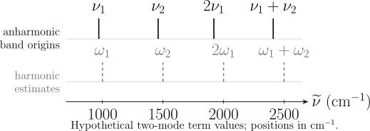
A hypothetical two-mode assignment. Solid sticks are anharmonic band origins; gray dashed sticks are the corresponding harmonic estimates. The displacement is not a universal red shift: its sign and size depend on the force field and state coupling. Stick heights are schematic and not intensities.

Worked two-mode assignment

Consider the term-value model

$$\begin{aligned} G(v_1,v_2) &= \sum_{i=1}^{2} \omega_i \left(v_i+\frac12\right) \\ &\quad + x_{11}\left(v_1+\frac12\right)^2 \\ &\quad + x_{22}\left(v_2+\frac12\right)^2 \\ &\quad + x_{12} \left(v_1+\frac12\right) \left(v_2+\frac12\right), \end{aligned}$$

with all constants in $\mathrm{cm}^{-1}$:

$$\begin{gathered} \omega_1=1000, \qquad \omega_2=1500, \\ x_{11}=-10, \qquad x_{22}=-15, \\ x_{12}=-20. \end{gathered}$$

Subtracting the ground-state term value gives

$$\begin{aligned} \widetilde\nu_1 &=970,\\ \widetilde\nu_2 &=1460,\\ \widetilde\nu_{2\nu_1} &=1920,\\ \widetilde\nu_{\nu_1+\nu_2} &=2410. \end{aligned}$$

The overtone is not $2\widetilde\nu_1$: here

$$2\widetilde\nu_1=1940 \mathrm{cm}^{-1},$$

whereas its calculated band origin is $1920\ \mathrm{cm}^{-1}$. Cross-mode anharmonicity and the different occupation-number dependence prevent simple multiplication of a measured fundamental.

Why overtones can appear

In the doubly idealized harmonic-plus-linear-dipole model, $0\to2$ vanishes because $Q_i$ changes the oscillator quantum number by one. Two mechanisms relax that result:

1. A quadratic dipole term contains $Q_i^2$, whose harmonic matrix element connects $v_i=0$ and $v_i=2$.
2. An anharmonic potential mixes harmonic states, so the exact vibrational eigenstates no longer carry pure $v_i$ labels.

An overtone can also borrow strength from a nearby bright fundamental. Its observability therefore contains information about both the dipole surface and vibrational coupling.

Temperature and hot bands

For nondegenerate harmonic levels in thermal equilibrium,

$$\frac{N_{v=1}}{N_{v=0}} = \exp\left( -\frac{hc\widetilde\nu}{k_{\mathrm B}T} \right).$$

Writing $c_2=hc/k_{\mathrm B}=1.4387769\ \mathrm{cm\,K}$ gives

$$\frac{N_1}{N_0} = \exp\left(-\frac{c_2\widetilde\nu}{T}\right).$$

Low-frequency modes can therefore generate visible hot bands at ordinary temperatures, while high-frequency bond stretches may remain overwhelmingly in $v=0$. Degeneracy and rotational populations must be included when a quantitative intensity ratio is required.

Connecting Spectra to Force Constants

Diatomic curvature from a harmonic wavenumber

For a diatomic coordinate with reduced mass $\mu$ and harmonic wavenumber $\omega_e$,

$$\Omega_e = 2\pi c\omega_e,$$

so the quadratic force constant is

$$k = \mu\Omega_e^2 = \mu(2\pi c\omega_e)^2.$$

The units must be consistent. If $c$ is in $\mathrm{cm\,s^{-1}}$ and $\omega_e$ in $\mathrm{cm}^{-1}$, their product is in $\mathrm{s}^{-1}$. For the hypothetical values

$$\begin{gathered} \mu=1.00\times10^{-26}\ \mathrm{kg}, \\ \omega_e=2000\ \mathrm{cm}^{-1}, \end{gathered}$$

one obtains

$$k\approx1.42\times10^3\ \mathrm{N\,m^{-1}}.$$

This $k$ is the curvature at equilibrium in the specified coordinate. It is not a dissociation energy and need not predict highly excited levels.

Why a fundamental is not enough by itself

If only the fundamental is observed, then the diatomic relation

$$\widetilde\nu_{1\leftarrow0} = \omega_e-2\omega_ex_e+\cdots$$

contains at least two unknown constants. A harmonic estimate may replace $\omega_e$ by the fundamental, but the resulting force constant is explicitly an effective approximation. Hot bands, overtones, isotope data, or a physically constrained potential can separate curvature from anharmonicity.

Polyatomic inverse problem

For a polyatomic molecule, observed harmonic frequencies constrain the eigenvalues of the mass-weighted Hessian. Eigenvalues alone do not reconstruct the entire matrix. Different force fields can share the same spectrum, especially when only a subset of modes is observed.

A useful force-field determination may combine:

• infrared and Raman band positions and intensities;
• isotope substitutions, which change $M$ while approximately preserving the Born–Oppenheimer force field;
• rotational constants and symmetry assignments;
• mode displacement vectors from electronic-structure calculations;
• overtone, combination, and resonance data; and
• an internal-coordinate force-field model with stated constraints.

Even then, individual “bond force constants” depend on the chosen internal coordinates and coupling terms. Normal-mode frequencies are observables or derived term values; a decomposition into local stretching, bending, and interaction constants is model-dependent.

Isotope substitution as a controlled perturbation

Within the Born–Oppenheimer approximation, isotopic substitution changes nuclear masses much more strongly than it changes the electronic potential. For an isolated diatomic harmonic mode,

$$\omega_e \propto \mu^{-1/2}.$$

For a polyatomic molecule, one must solve the full mass-weighted eigenproblem; there is generally no single reduced mass attached to a collective mode. Isotopic shifts are powerful because they test mode assignments and constrain eigenvectors as well as frequencies. Deviations from simple mass scaling can also expose vibrational mixing, nonadiabatic corrections, or inconsistent assignments.

Harmonic calculations and scale factors

An electronic-structure frequency calculation usually diagonalizes a mass-weighted Hessian at an optimized geometry. Its output is a set of harmonic wavenumbers. Experiment commonly reports fundamentals. Their difference combines at least two effects:

1. the physical anharmonic correction; and
2. error in the electronic structure, basis set, geometry, and numerical Hessian.

Empirical scale factors can reduce average discrepancies for a declared method, basis, molecular class, and target property. They do not turn a harmonic calculation into an anharmonic Hamiltonian, resolve resonances, or provide a molecule-specific uncertainty automatically. A scale factor fitted to fundamentals should not be reused silently for zero-point energies or transition intensities.

Reading Experimental Spectra

Gas, liquid, and solid samples answer different questions

Environment	Typical spectral consequences	Interpretation caution
Dilute gas	Rotational fine structure may be resolved; isolated-molecule quantum numbers are useful	Doppler, pressure, hyperfine, and unresolved rovibrational structure still matter
Liquid or solution	Rotation is strongly interrupted; bands broaden and solvent shifts appear	Peak positions and widths depend on concentration, solvent, temperature, and hydrogen bonding
Matrix or molecular solid	Site splitting, crystal fields, phonon coupling, and collective modes may appear	Free-molecule point-group labels can be reduced by the environment
Periodic solid	Zone-center optical phonons and crystal momentum replace an isolated-molecule mode picture	A molecular normal-mode assignment may be only an approximate local description

Comparing a gas-phase computed harmonic wavenumber directly with a broad solution-phase peak can be useful for orientation, but it is not a like-for-like test of an isolated molecular Hamiltonian.

High-resolution vibrational bands are rovibrational

Molecules normally rotate while vibrating. A gas-phase infrared transition therefore connects rovibrational states, not pure vibrational states. Branch structure can reveal the band origin and vibration-dependent rotational constants, while unresolved rotation can shift the apparent envelope maximum. The P/Q/R hierarchy and Coriolis complications are developed in Rovibrational Coupling.

Peak position, area, and width carry different information

• Position constrains an energy difference after shifts and unresolved structure are modeled.
• Integrated area constrains a population-weighted transition strength under a declared normalization.
• Width and shape constrain lifetimes, collisions, inhomogeneity, instrumental response, and unresolved components.

These observables should not be interchanged. A broader band can have a lower peak while retaining the same integrated area. Line Shapes and Broadening develops that distinction.

Databases and line lists

A line list may tabulate wavenumbers, lower-state energies, Einstein coefficients, statistical weights, pressure-broadening parameters, and temperature-dependent intensities. Before using one, check:

• isotopologue and isotopic-abundance convention;
• vacuum versus medium wavenumber;
• reference temperature and partition-function convention;
• whether positions are measured, fitted, or predicted;
• uncertainty and quantum-number completeness; and
• whether the file contains discrete lines or a measured cross section.

For example, HITRAN line intensity incorporates the lower-state population, stimulated-emission factor, partition function, and a terrestrial isotopic abundance convention. It is not simply $|M_{ul}|^2$. The NIST Chemistry WebBook provides evaluated and compiled vibrational data for many species, but each species page must still be read for data provenance and phase.

Assignment Workflow

A defensible assignment can be organized as follows.

1. Record metadata. State sample identity, isotopic composition, phase, temperature, pressure or matrix, path length, resolution, polarization, and calibration.
2. Process conservatively. Preserve the raw spectrum. Document baseline, atmospheric subtraction, apodization, smoothing, and deconvolution.
3. Identify reproducible features. Report positions, areas, widths, and uncertainties rather than only a peak-picked image.
4. Count and classify modes. Use molecular geometry and symmetry to predict mode number, degeneracy, and first-order activity.
5. Generate zeroth-order estimates. Use harmonic calculations, isotope shifts, known functional-group ranges, or an effective Hamiltonian without presenting them as final assignments.
6. Search for families. Fundamentals, hot bands, overtones, combinations, rotational branches, isotope partners, and temperature trends should form mutually consistent patterns.
7. Test interactions. Near-degenerate same-symmetry states, anomalous shifts, and redistributed intensity signal possible resonance.
8. Fit with withheld checks. Use the smallest physically motivated model, inspect signed residuals, and test predictions against lines or isotopes not used in the fit.
9. Separate result from inference. Distinguish measured centers, assigned quantum numbers, fitted constants, and model-derived force constants.

One coincident peak is weak evidence. A network of positions, intensities, symmetry, isotope shifts, and temperature behavior is much stronger.

Common Mistakes

Mistake	Why it fails	Better practice
Calling every peak a normal-mode frequency	Peaks can be hot bands, overtones, combinations, rotational components, impurities, or artifacts	Reserve “normal-mode frequency” for a declared harmonic model and assign measured transitions explicitly
Setting the harmonic wavenumber equal to the fundamental	Anharmonicity shifts $1\leftarrow0$ from the local-curvature value	Fit anharmonic constants or label the replacement as an approximation
Assuming a permanent dipole guarantees every IR band	Activity depends on $\partial\boldsymbol\mu/\partial Q_i$, not only $\boldsymbol\mu_e$	Evaluate transition moments and symmetry mode by mode
Declaring an absent band forbidden	Population, overlap, weak intensity, detector response, and selection rules all affect visibility	State a detection limit and the operator/symmetry approximation
Taking $2\widetilde\nu_i$ as the overtone position	Diagonal and cross-anharmonicities differ among occupation patterns	Use term-value differences and test for resonances
Assigning one force constant to each peak	Polyatomic frequencies are eigenvalues of a coupled mass-weighted force field	State the coordinate system and fit coupled force constants with additional constraints
Comparing a scaled calculation and experiment without metadata	Scale factors are method-, basis-, dataset-, and target-dependent	Cite the factor, training set, uncertainty, and whether the target is a fundamental or zero-point energy
Treating a solution peak as a gas-phase band origin	Solvation and unresolved structure shift and broaden the feature	Match phase and conditions or model the environmental shift

Key Takeaways

• Harmonic normal modes provide the first language of vibrational assignment, not exact observed band positions.
• Infrared activity is controlled by a transition dipole; at first order it requires a nonzero dipole derivative along the mode.
• Anharmonic potential and dipole surfaces are distinct sources of shifted levels and nominally forbidden intensity.
• Fundamentals, hot bands, overtones, and combinations are state-to-state labels and must be separated from unresolved rotational or environmental structure.
• A diatomic harmonic wavenumber gives a local force constant once the reduced mass is known; a polyatomic spectrum does not uniquely determine a full force field from eigenvalues alone.
• Reliable assignments combine symmetry, isotope shifts, populations, intensities, residuals, and experimental metadata.

Exercises

Exercise 1: Fundamental and hot-band spacing

A diatomic molecule has

$$\begin{gathered} \widetilde\nu_{1\leftarrow0}=2140\ \mathrm{cm}^{-1}, \\ \widetilde\nu_{2\leftarrow1}=2100\ \mathrm{cm}^{-1}. \end{gathered}$$

Using the two-term anharmonic model, determine $\omega_e$ and $\omega_ex_e$. Predict the $2\leftarrow0$ overtone position.

Solution

The adjacent intervals are

$$\begin{aligned} \widetilde\nu_{1\leftarrow0} &=\omega_e-2\omega_ex_e,\\ \widetilde\nu_{2\leftarrow1} &=\omega_e-4\omega_ex_e. \end{aligned}$$

Their difference gives

$$2\omega_ex_e = 40\ \mathrm{cm}^{-1},$$

so

$$\omega_ex_e=20\ \mathrm{cm}^{-1}, \qquad \omega_e=2180\ \mathrm{cm}^{-1}.$$

The ground-state overtone is

$$\begin{aligned} \widetilde\nu_{2\leftarrow0} &=2\omega_e-6\omega_ex_e\\ &=4240\ \mathrm{cm}^{-1}. \end{aligned}$$

It is $40\ \mathrm{cm}^{-1}$ below twice the fundamental, illustrating why an overtone is not located by simple multiplication.

Exercise 2: Force constant and units

A diatomic has reduced mass $\mu=1.00\times10^{-26}\ \mathrm{kg}$ and harmonic wavenumber $\omega_e=2000\ \mathrm{cm}^{-1}$. Calculate its harmonic force constant. Use $c=2.99792458\times10^{10}\ \mathrm{cm\,s^{-1}}$.

Solution

First convert the spectroscopic constant to angular frequency:

$$\begin{aligned} \Omega_e &=2\pi c\omega_e\\ &=2\pi (2.99792458\times10^{10}) (2000)\\ &\approx3.7673\times10^{14}\ \mathrm{s}^{-1}. \end{aligned}$$

Then

$$\begin{aligned} k &=\mu\Omega_e^2\\ &=(1.00\times10^{-26}) (3.7673\times10^{14})^2\\ &\approx1.42\times10^3\ \mathrm{N\,m^{-1}}. \end{aligned}$$

Using $c$ in $\mathrm{m\,s^{-1}}$ while leaving $\omega_e$ in $\mathrm{cm}^{-1}$ would introduce an error of $10^4$ in $k$.

Exercise 3: Mode count and degeneracy

Count the vibrational coordinates and distinct harmonic frequencies expected for water and linear carbon dioxide. Explain why the two numbers differ for carbon dioxide.

Solution

Water is nonlinear with $N=3$, so it has

$$3N-6=3$$

vibrational coordinates and three distinct frequencies in the absence of an accidental degeneracy.

Carbon dioxide is linear, so it has

$$3N-5=4$$

vibrational coordinates. Its two perpendicular bending coordinates are degenerate in the isolated linear molecule. It therefore has four coordinates but three distinct harmonic frequencies: symmetric stretch, doubly degenerate bend, and antisymmetric stretch.

Exercise 4: Infrared activity without a permanent dipole

Carbon dioxide has no equilibrium dipole moment. Why can its antisymmetric stretch absorb infrared light while its symmetric stretch is inactive at first electric-dipole order?

Solution

Infrared activity depends on the transition dipole, whose leading vibrational term is controlled by

$$\left( \frac{\partial\boldsymbol\mu}{\partial Q_i} \right)_e.$$

During the antisymmetric stretch, the two bond contributions cease to cancel instantaneously, so a dipole component changes along the mode and the derivative is nonzero. During the symmetric stretch, inversion symmetry is preserved and the electric-dipole derivative vanishes in the ideal molecule. The equilibrium value $\boldsymbol\mu_e=0$ does not decide either result by itself.

Exercise 5: Mechanical and electrical anharmonicity

For a one-dimensional mode, suppose the potential is exactly harmonic but the dipole function contains a quadratic term. Can the $2\leftarrow0$ transition appear? Conversely, can it appear with a linear dipole function and an anharmonic potential?

Solution

Yes in both cases.

With harmonic states and

$$\mu(Q) = \mu_e+\mu'_eQ+\frac12\mu''_eQ^2+\cdots,$$

the matrix element

$$\langle2|Q^2|0\rangle$$

is nonzero, so the quadratic dipole term gives electrical-anharmonic overtone intensity.

With a linear dipole but an anharmonic potential, the exact eigenstates are mixtures of harmonic number states. The matrix element of $Q$ between the mixed ground and second excited states can then be nonzero. This is mechanical anharmonicity. An observed overtone may contain both contributions.

Exercise 6: Two-mode combination band

Use the two-mode constants from the worked example to verify the combination band origin for $(v_1,v_2)=(1,1)\leftarrow(0,0)$. Compare it with both the harmonic sum and the sum of the two fundamentals.

Solution

For the combination state, the diagonal terms change by $2x_{11}$ and $2x_{22}$, while the $x_{12}$ product changes from $1/4$ to $9/4$, giving $2x_{12}$. Thus

$$\begin{aligned} \widetilde\nu_{\nu_1+\nu_2} &= \omega_1+\omega_2 +2x_{11}+2x_{22}+2x_{12}\\ &=1000+1500-20-30-40\\ &=2410\ \mathrm{cm}^{-1}. \end{aligned}$$

The harmonic sum is

$$\omega_1+\omega_2=2500\ \mathrm{cm}^{-1},$$

whereas the sum of fundamentals is

$$970+1460=2430\ \mathrm{cm}^{-1}.$$

Neither equals the combination origin because its cross-anharmonic occupation factor differs from those in the separate fundamentals.

Exercise 7: Thermal population of a low-frequency mode

Estimate $N_1/N_0$ at $T=300\ \mathrm K$ for a nondegenerate mode with $\widetilde\nu=500\ \mathrm{cm}^{-1}$. Use $c_2=1.4387769\ \mathrm{cm\,K}$. What does the result suggest about hot bands?

Solution

The Boltzmann ratio is

$$\begin{aligned} \frac{N_1}{N_0} &= \exp\left[-\frac{(1.4387769)(500)}{300}\right]\\ &=\exp(-2.39796)\\ &\approx0.091. \end{aligned}$$

About nine percent as many molecules occupy $v=1$ as $v=0$ before rotational and degeneracy factors are included. A $2\leftarrow1$ hot band may therefore be observable if its transition moment and spectral separation are favorable. The ratio would be much smaller for a high-frequency stretching mode at the same temperature.

Exercise 8: Force-field identifiability

A nonlinear four-atom molecule has six accurately measured fundamental band origins. Do those six numbers uniquely determine its full Cartesian Hessian? Give three kinds of additional information that can make a force-field fit more informative.

Solution

No. The six fundamentals are anharmonic transition energies, not even the six harmonic Hessian eigenvalues without correction. Eigenvalues alone also do not determine all matrix elements or eigenvectors of the mass-weighted Hessian. The inverse problem remains model-dependent.

Useful additional constraints include any three of:

• isotope shifts from several substitutions;
• infrared and Raman symmetry assignments and polarization data;
• calculated normal-mode eigenvectors and a computed quadratic force field;
• overtone and combination-band term values that constrain anharmonic constants;
• rotational constants or structural constraints; and
• an internal-coordinate force-field model with physically justified sparsity or symmetry relations.

The fitted force constants must be reported with their coordinate convention and model uncertainty.

Cross-Links

• Spectroscopy
• Transition Rates
• Absorption and Emission
• Line Shapes and Broadening
• Selection Rules in Spectroscopy
• Rotational Spectroscopy
• Infrared Spectroscopy
• Raman Spectroscopy
• Vibrations of Diatomics
• Normal Modes of Polyatomics
• Rovibrational Coupling
• Molecular Symmetry
• Quantum Harmonic Oscillator
• Oscillator as a Universal Local Model
• Anharmonic Oscillator
• Selection Rules and Transition Rates
• Molecular Physics
• Selection Rule Tables for IR, Raman, and rovibrational quick reference

References

• E. B. Wilson Jr., J. C. Decius, and P. C. Cross, Molecular Vibrations: The Theory of Infrared and Raman Vibrational Spectra, McGraw–Hill, 1955; Dover reprint, 1980.
• G. Herzberg, Molecular Spectra and Molecular Structure. I. Spectra of Diatomic Molecules, 2nd ed., Van Nostrand, 1950.
• G. Herzberg, Molecular Spectra and Molecular Structure. II. Infrared and Raman Spectra of Polyatomic Molecules, Van Nostrand, 1945.
• P. F. Bernath, Spectra of Atoms and Molecules, 5th ed., Oxford University Press, 2025, doi:10.1093/oso/9780197754498.001.0001.
• P. R. Bunker and P. Jensen, Molecular Symmetry and Spectroscopy, 2nd ed., NRC Research Press, 1998.
• D. Papoušek and M. R. Aliev, Molecular Vibrational-Rotational Spectra, Elsevier, 1982.
• P. M. Morse, “Diatomic Molecules According to the Wave Mechanics. II. Vibrational Levels,” Physical Review 34, 57–64 (1929), doi:10.1103/PhysRev.34.57.
• J. L. Dunham, “The Energy Levels of a Rotating Vibrator,” Physical Review 41, 721–731 (1932), doi:10.1103/PhysRev.41.721.
• V. Barone, “Anharmonic Vibrational Properties by a Fully Automated Second-Order Perturbative Approach,” Journal of Chemical Physics 122, 014108 (2005), doi:10.1063/1.1824881.
• International Union of Pure and Applied Chemistry, “normal mode”, Compendium of Chemical Terminology, 5th ed., online version 5.0.0, 2025, doi:10.1351/goldbook.08648.
• K. K. Irikura, R. D. Johnson III, and R. N. Kacker, “Uncertainties in Scaling Factors for Ab Initio Vibrational Frequencies,” Journal of Physical Chemistry A 109, 8430–8437 (2005), doi:10.1021/jp052793n.
• NIST Computational Chemistry Comparison and Benchmark Database, Vibrational Frequency Scaling Factors, accessed 2026-07-22.
• NIST Chemistry WebBook, SRD 69, Vibrational and electronic energy levels, accessed 2026-07-22.
• HITRANonline, Units and Definitions and Quantum Notation, accessed 2026-07-22.