Vibrations of Diatomics

A diatomic vibration is quantum motion in the internuclear separation $R$, not a pair of nuclei following a sharply defined classical trajectory. On an isolated electronic potential, the lowest vibrational states usually sample a narrow neighborhood of an equilibrium separation $R_e$. The local curvature then produces an oscillator scale. Real molecular wells are asymmetric and dissociate, however, so their level spacings decrease with excitation and their spectra carry information beyond a single force constant.

Three distinctions organize a trustworthy treatment:

• the potential-energy curve and nuclear masses are inputs to a nuclear Hamiltonian;
• vibrational term values are eigenvalue differences or fitted effective parameters, not a direct image of the potential;
• infrared activity belongs to a transition moment, not merely to the existence of a vibration or a permanent dipole.

The harmonic oscillator is therefore the beginning of molecular vibration, not its endpoint.

Canonical Scope

This page is the canonical home for:

• reducing one-surface diatomic nuclear motion to a radial vibrational problem;
• converting potential curvature and reduced mass into angular-frequency, frequency, and wavenumber conventions;
• zero-point widths, isotope scaling, and leading Dunham mass scaling;
• anharmonic vibrational term values, interval contraction, zero-point energy, and dissociation conventions;
• the Morse potential as an exactly solvable finite-well model and as a deliberately limited extrapolation;
• electric-dipole vibrational selection rules from the molecular dipole function;
• fundamentals, hot bands, overtones, and the inference chain from infrared data to molecular parameters.

Quantum Harmonic Oscillator owns the exact oscillator spectrum and wavefunctions. Oscillator as a Universal Local Model owns the general Taylor-expansion logic near stable equilibria. Anharmonic Oscillator owns generic perturbative, variational, and numerical methods for anharmonic model Hamiltonians. Here those tools are applied to a molecular bond, with spectroscopic conventions, dissociation physics, isotope dependence, and transition moments.

From a Molecular Hamiltonian to One Coordinate

Assumptions behind the radial problem

Consider two nuclei $A$ and $B$ on one isolated adiabatic electronic surface. Remove overall center-of-mass translation and define

$$\mathbf R = \mathbf R_B-\mathbf R_A, \qquad R=\lvert\mathbf R\rvert,$$

with nuclear reduced mass

$$\mu = \frac{M_AM_B}{M_A+M_B}.$$

For a closed-shell electronic $\Sigma$ state, after neglecting electronic angular momentum, spin couplings, and nonadiabatic channel mixing, the reduced radial equation is

$$\begin{aligned} \Bigg[ &- \frac{\hbar^2}{2\mu} \frac{d^2}{dR^2} + \frac{\hbar^2J(J+1)} {2\mu R^2} \\ &+ U(R) \Bigg] u_{vJ}(R) = E_{vJ}u_{vJ}(R). \end{aligned}$$

The reduced wavefunction obeys

$$u_{vJ}(0)=0, \qquad \int_0^\infty \lvert u_{vJ}(R)\rvert^2\,dR =1.$$

Here $U(R)$ may be a Born–Oppenheimer potential alone or a declared effective curve containing diagonal adiabatic corrections. The distinction matters at high accuracy. Born–Oppenheimer in Molecules derives this hierarchy and its corrections.

This page first sets $J=0$ to isolate vibration:

$$\left[ - \frac{\hbar^2}{2\mu} \frac{d^2}{dR^2} + U(R) \right] u_v(R) = E_vu_v(R).$$

Rotation is not absent from real gas-phase infrared spectra. It is temporarily projected out so that the vibrational structure can be identified cleanly. Rotations of Molecules owns the rotational effective theory.

Energy-zero and dissociation conventions

Choose the potential minimum as zero:

$$U(R_e)=0, \qquad U'(R_e)=0.$$

For a bound electronic state that correlates with a separated-fragment channel,

$$D_e = U(\infty)-U(R_e)$$

is the well depth measured from the equilibrium minimum. The dissociation energy from the lowest vibrational state is instead

$$D_0 = U(\infty)-E_0.$$

Within a single uncoupled vibrational curve,

$$D_0=D_e-E_0.$$

When energies are divided by $hc$, use tildes:

$$\widetilde D_e=\frac{D_e}{hc}, \qquad \widetilde D_0=\frac{D_0}{hc}.$$

Confusing $D_e$ with $D_0$ discards the vibrational zero-point energy. Confusing either with a thermochemical bond energy can also hide electronic degeneracies, fine structure, thermal averaging, and the identity of the dissociation products.

Harmonic Approximation Near Equilibrium

Curvature defines the leading model

Let

$$q=R-R_e.$$

For a smooth potential near a stable minimum,

$$\begin{aligned} U(R) = {}& \frac12kq^2 + \frac{1}{3!}k_3q^3 \\ &+ \frac{1}{4!}k_4q^4 +\cdots, \end{aligned}$$

where

$$k = \left. \frac{d^2U}{dR^2} \right|_{R_e} >0.$$

Retaining only the quadratic term gives

$$\hat H_{\mathrm{vib}}^{(2)} = - \frac{\hbar^2}{2\mu} \frac{d^2}{dq^2} + \frac12kq^2.$$

The molecular coordinate has the exact domain $q\in(-R_e,\infty)$. The harmonic model extends it to the full real line. That extension is accurate only when the relevant wavefunction is exponentially small near $R=0$ and well localized far from dissociation.

Frequency notation without ambiguity

Molecular spectroscopy and oscillator mechanics use similar symbols for different quantities. This page reserves $\Omega_e$ for angular frequency:

$$\Omega_e = \sqrt{\frac{k}{\mu}}.$$

The corresponding ordinary frequency and harmonic wavenumber are

$$\nu_e = \frac{\Omega_e}{2\pi}, \qquad \widetilde\nu_e = \frac{\Omega_e}{2\pi c}.$$

In conventional diatomic spectroscopy, the wavenumber $\widetilde\nu_e$ is normally written $\omega_e$. Thus

$$\omega_e \equiv \frac{\Omega_e}{2\pi c}$$

has units of $\mathrm{cm}^{-1}$ when $c$ and the length unit are chosen consistently. It is not an angular frequency despite the symbol.

Symbol on this page	Meaning	Typical unit
$\Omega_e$	angular frequency $\sqrt{k/\mu}$	$\mathrm{rad\,s^{-1}}$
$\nu_e$	ordinary frequency $\Omega_e/(2\pi)$	$\mathrm{Hz}$
$\omega_e$	conventional spectroscopic harmonic constant	$\mathrm{cm}^{-1}$
$G(v)$	vibrational term value $E_v/(hc)$ relative to a stated zero	$\mathrm{cm}^{-1}$

The conversion back to a force constant is

$$k = \mu \left( 2\pi c\omega_e \right)^2.$$

Using an observed fundamental band position in this equation silently treats an anharmonic transition interval as the harmonic constant. That substitution is often numerically close for low levels but is conceptually wrong.

Harmonic levels and wavefunction scale

Borrowing the canonical oscillator solution,

$$E_v^{(2)} = \hbar\Omega_e \left( v+\frac12 \right), \qquad v=0,1,2,\ldots.$$

In term-value units,

$$G^{(2)}(v) = \omega_e \left( v+\frac12 \right).$$

The natural oscillator length is

$$\ell_e = \sqrt{ \frac{\hbar}{\mu\Omega_e} }.$$

For level $v$,

$$\langle q\rangle_v=0, \qquad \langle q^2\rangle_v = \ell_e^2 \left( v+\frac12 \right).$$

The ground-state root-mean-square displacement is therefore

$$q_{\mathrm{rms},0} = \sqrt{ \frac{\hbar}{2\mu\Omega_e} } = \frac{\ell_e}{\sqrt2}.$$

This width is a probability-distribution scale. It is not the amplitude of a nucleus executing a classical orbit. In an anharmonic well, $\langle q\rangle_v$ generally becomes positive because the wavefunction samples farther toward the softer dissociation side.

A local validity test

At a characteristic displacement $q_\star$, compare higher terms with the quadratic energy:

$$\epsilon_3(q_\star) \sim \left| \frac{k_3q_\star}{3k} \right|, \qquad \epsilon_4(q_\star) \sim \left| \frac{k_4q_\star^2}{12k} \right|.$$

For the ground state, $q_\star\sim\ell_e$ is a useful first estimate. For excited states, the sampled width grows approximately as $\ell_e\sqrt{v+1/2}$, so a harmonic approximation that is excellent at $v=0$ can fail badly at larger $v$.

Curvature alone determines only the local oscillator scale. It does not determine the global well depth, the number of bound states, or the dissociation products.

Reduced Mass and Isotope Scaling

What isotopic substitution changes

In the strict Born–Oppenheimer approximation, isotopologues share the same electronic potential $U(R)$ but have different nuclear masses. Holding the curvature fixed gives

$$\Omega_e \propto \mu^{-1/2}, \qquad \omega_e \propto \mu^{-1/2}.$$

The zero-point energy and ground-state width scale as

$$E_{\mathrm{zp}} \propto \mu^{-1/2}, \qquad q_{\mathrm{rms},0} \propto \mu^{-1/4}.$$

Thus a heavier isotopologue has:

• a smaller vibrational spacing;
• a smaller zero-point energy;
• a narrower low-lying vibrational distribution;
• usually a larger $D_0$ for the same $D_e$, because less energy is already stored in zero-point motion.

These statements are leading mass laws. At spectroscopic precision, diagonal adiabatic corrections, nonadiabatic effective masses, nuclear size, and hyperfine structure produce deviations.

A hydrogen-chloride estimate

Using atomic masses

$$\begin{aligned} m(^{1}\mathrm H)&=1.007825\,\mathrm u,\\ m(^{2}\mathrm H)&=2.014102\,\mathrm u,\\ m(^{35}\mathrm{Cl})&=34.968853\,\mathrm u, \end{aligned}$$

gives approximately

$$\begin{aligned} \mu(^{1}\mathrm H^{35}\mathrm{Cl}) &=0.979593\,\mathrm u,\\ \mu(^{2}\mathrm H^{35}\mathrm{Cl}) &=1.904413\,\mathrm u. \end{aligned}$$

The common-surface harmonic prediction is

$$\frac{ \omega_e(^{2}\mathrm H^{35}\mathrm{Cl}) }{ \omega_e(^{1}\mathrm H^{35}\mathrm{Cl}) } \approx \sqrt{ \frac{0.979593}{1.904413} } =0.7172.$$

This ratio is a model prediction, not an exact isotope identity. Comparing several constants and isotopologues is one way to expose corrections beyond the leading Born–Oppenheimer picture.

Dunham organization

A widely used effective expansion combines vibration and rotation:

$$\frac{E_{vJ}}{hc} = \sum_{k,l} Y_{kl} \left( v+\frac12 \right)^k \left[ J(J+1) \right]^l.$$

For pure vibration,

$$Y_{10}\approx\omega_e, \qquad Y_{20}\approx-\omega_ex_e,$$

where $\omega_ex_e$ denotes the product $\omega_e x_e$. In the leading Born–Oppenheimer mass scaling,

$$Y_{kl} \propto \mu^{-(k/2+l)}.$$

Examples are

$$\begin{aligned} Y_{10} &\propto \mu^{-1/2}, \\ Y_{20} &\propto \mu^{-1}, \\ Y_{01} &\propto \mu^{-1}. \end{aligned}$$

The expansion is an effective representation over a fitted range. Its coefficients can include perturbations, and a finite polynomial in $v+1/2$ should not be extrapolated casually to dissociation.

Anharmonic Vibrational Structure

Why real intervals contract

A molecular bond is steep under compression and soft toward dissociation. The cubic term represents the leading local asymmetry; quartic and higher terms further change the level pattern. The resulting eigenstates are not exact harmonic number states, and adjacent spacings are no longer equal.

Spectroscopists organize the vibrational term values as

$$\begin{aligned} G(v) = {}& \omega_e \left( v+\frac12 \right) \\ &- \omega_ex_e \left( v+\frac12 \right)^2 \\ &+ \omega_ey_e \left( v+\frac12 \right)^3 +\cdots. \end{aligned}$$

The products $\omega_ex_e$ and $\omega_ey_e$ are each reported in wavenumber units. For the common case $\omega_ex_e>0$, the quadratic correction lowers high levels and makes the ladder contract.

Keeping two terms,

$$\begin{aligned} \widetilde\nu_{v+1\leftarrow v} &= G(v+1)-G(v) \\ &= \omega_e - 2\omega_ex_e(v+1). \end{aligned}$$

Therefore

$$\begin{aligned} \widetilde\nu_{1\leftarrow0} &= \omega_e-2\omega_ex_e,\\ \widetilde\nu_{2\leftarrow1} &= \omega_e-4\omega_ex_e,\\ \widetilde\nu_{2\leftarrow0} &= 2\omega_e-6\omega_ex_e. \end{aligned}$$

The first line is the fundamental, the second is a hot-band interval, and the third is the first overtone interval. An overtone position is not twice the observed fundamental once anharmonicity is present.

Zero-point energy

The term-value expansion gives

$$G(0) = \frac12\omega_e - \frac14\omega_ex_e + \frac18\omega_ey_e +\cdots.$$

Consequently,

$$\widetilde D_0 = \widetilde D_e-G(0)$$

within the declared one-surface model. A measured spectrum gives level differences most directly; obtaining $G(0)$ and the dissociation limit requires a model, additional bands, or independent threshold information.

Measured HCl levels

The NIST-JANAF critical evaluation tabulates the following $^{1}\mathrm H^{35}\mathrm{Cl}$ ground-state vibrational term differences after resolving rotation:

$v$	$G(v)-G(0)$ ($\mathrm{cm}^{-1}$)	Adjacent spacing ($\mathrm{cm}^{-1}$)
0	0.00	—
1	2885.36	2885.36
2	5666.79	2781.43
3	8345.05	2678.26
4	10920.63	2575.58
5	13393.64	2473.01

The nearly $104\,\mathrm{cm}^{-1}$ decrease per step at low $v$ is the operational signature of leading anharmonicity. The progression is not exactly linear, so higher-order terms and a global potential are needed for precision or near-dissociation work.

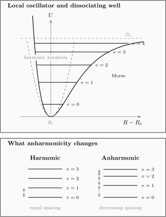
The harmonic parabola matches only the local curvature at $R_e$ and has an infinite equally spaced ladder. A dissociating well is asymmetric, supports finitely many bound levels, and generally has decreasing adjacent spacings. The drawn levels are schematic rather than fitted to a particular molecule.

The Morse Potential

Definition and local curvature

The Morse model replaces the global parabola by

$$\begin{aligned} U_{\mathrm M}(R) &= D_e \left[ 1-e^{-a(R-R_e)} \right]^2, \\ a&>0. \end{aligned}$$

It has

$$U_{\mathrm M}(R_e)=0, \qquad \lim_{R\to\infty} U_{\mathrm M}(R)=D_e,$$

and becomes strongly repulsive under compression. Its equilibrium curvature is

$$k=2D_ea^2,$$

so the local angular frequency is

$$\Omega_e = a \sqrt{ \frac{2D_e}{\mu} }.$$

The three parameters $R_e$, $D_e$, and $a$ therefore encode the minimum position, well depth, and local stiffness.

Exact energy levels

Define

$$\lambda = \frac{ \sqrt{2\mu D_e} }{ a\hbar } = \frac{2D_e}{\hbar\Omega_e}.$$

The bound-state energies relative to the minimum are

$$\begin{aligned} E_v = {}& \hbar\Omega_e \left( v+\frac12 \right) \\ &- \frac{ \hbar^2\Omega_e^2 }{ 4D_e } \left( v+\frac12 \right)^2. \end{aligned}$$

Equivalently,

$$E_v = D_e - \frac{a^2\hbar^2}{2\mu} \left( \lambda-v-\frac12 \right)^2.$$

Normalizable bound states satisfy

$$v+\frac12<\lambda.$$

Unlike the harmonic oscillator, the Morse potential supports a finite number of vibrational levels. Their spacings approach zero as the formal dissociation limit is approached.

In spectroscopic units, the exact Morse spectrum has the two-term form

$$G_{\mathrm M}(v) = \omega_e \left( v+\frac12 \right) - \omega_ex_e \left( v+\frac12 \right)^2,$$

with the special Morse relation

$$\omega_ex_e = \frac{\omega_e^2} {4\widetilde D_e}.$$

Thus

$$\widetilde D_e^{(\mathrm M)} = \frac{\omega_e^2} {4\omega_ex_e}.$$

This inversion is exact only if the entire potential is Morse. For a real molecule, $\omega_e$ and $\omega_ex_e$ are low-energy local data; they do not generally determine the true asymptote.

What the model gets right

The Morse model improves on a global parabola by providing:

• an asymmetric well;
• decreasing level spacings;
• a finite dissociation energy;
• a finite bound-state ladder;
• analytic eigenvalues and wavefunctions;
• a transparent connection among curvature, anharmonicity, and depth.

It is therefore an excellent reasoning model and a useful basis for approximate calculations.

What the model gets wrong

For neutral separated fragments, the true long-range attraction usually has an inverse-power form such as

$$D_e-U(R) \sim \frac{C_6}{R^6} + \frac{C_8}{R^8} +\cdots,$$

whereas the Morse tail approaches its asymptote exponentially. Real potentials can also contain avoided crossings, multiple electronic channels, relativistic asymptotes, and short-range structure that three parameters cannot reproduce.

Consequences include:

• low-lying constants may fit well while $D_e$ is badly biased;
• the predicted number and placement of near-threshold states can be wrong;
• an exact Morse relation among constants is not a universal molecular identity;
• a fitted Morse curve should not be assigned uncertainty outside its calibration window without independent validation.

HCl as an extrapolation stress test

The NIST Chemistry WebBook compilation gives for the ground state of $^{1}\mathrm H^{35}\mathrm{Cl}$

$$\begin{aligned} \omega_e &= 2990.9463\,\mathrm{cm}^{-1}, \\ \omega_ex_e &= 52.8186\,\mathrm{cm}^{-1}. \end{aligned}$$

Treating those two local constants as an exact Morse spectrum predicts

$$\widetilde D_e^{(\mathrm M)} \approx 42342\,\mathrm{cm}^{-1}.$$

Using the corresponding two-term zero-point value gives

$$\widetilde D_0^{(\mathrm M)} \approx 40860\,\mathrm{cm}^{-1}.$$

The NIST-JANAF evaluation instead gives approximately

$$\widetilde D_0 \approx 35760\,\mathrm{cm}^{-1}$$

and identifies $v=19$ as the last bound vibrational level. The two-constant Morse extrapolation would allow levels through $v=27$. The discrepancy is not a failure of the measured low-energy constants. It is a failure of an overly rigid global model.

Vibrational Selection Rules

The transition moment is the central object

In the electric-dipole approximation, light couples through

$$\hat H'(t) = - \hat{\boldsymbol\mu} \mathbin{\boldsymbol\cdot} \mathbf E(t).$$

After projecting onto one electronic state and separating rotational factors, the vibrational transition moment contains

$$M_{v'v} = \int_0^\infty u_{v'}^*(R) \mu(R) u_v(R)\,dR,$$

where $\mu(R)$ is the relevant body-fixed electric-dipole function. A nonzero energy difference is not enough; absorption requires a nonzero matrix element for the actual interaction operator.

Expand the dipole function near equilibrium:

$$\mu(R) = \mu_e + \mu_e'q + \frac12\mu_e''q^2 +\cdots.$$

The constant term contributes

$$\mu_e \langle v'|v\rangle = \mu_e\delta_{v'v},$$

so a permanent dipole by itself cannot connect two orthogonal vibrational levels.

Harmonic fundamental rule

Write

$$q = q_{\mathrm{zp}} \left( a+a^\dagger \right), \qquad q_{\mathrm{zp}} = \sqrt{ \frac{\hbar}{2\mu\Omega_e} }.$$

Then

$$\langle v+1|q|v\rangle = q_{\mathrm{zp}} \sqrt{v+1},$$

and the linear dipole term gives

$$\Delta v=\pm1.$$

For absorption from a low-temperature sample, the dominant harmonic transition is usually

$$v=0\longrightarrow1.$$

Its leading vibrational amplitude is

$$M_{10} \approx \mu_e'q_{\mathrm{zp}}.$$

The mode is electric-dipole infrared active in this approximation only if

$$\mu_e' \ne0.$$

The relevant condition is a changing dipole moment, not merely a nonzero equilibrium dipole.

Overtones and hot bands

The quadratic dipole term has

$$\langle v'|q^2|v\rangle\ne0$$

for $\Delta v=0,\pm2$ in the harmonic basis. It can therefore drive a first overtone even when the potential remains harmonic. Conversely, an anharmonic potential mixes harmonic number states, allowing the linear dipole term to acquire matrix elements beyond $\Delta v=\pm1$.

Real overtone intensity can arise from both:

• electrical anharmonicity: nonlinear dependence of $\mu(R)$ on $R$;
• mechanical anharmonicity: nonquadratic $U(R)$ and the resulting mixed wavefunctions.

A hot band originates from a thermally populated excited vibrational level, such as $v=1\to2$. Its presence depends on temperature and population as well as on the transition moment.

The word forbidden should always be qualified. A vanishing leading electric-dipole matrix element does not exclude electric-quadrupole, magnetic-dipole, Raman, collision-induced, multiphoton, or symmetry-breaking processes.

Homonuclear and heteronuclear diatomics

For an isolated homonuclear diatomic in a nondegenerate electronic state, inversion and nuclear-exchange symmetry force the permanent electric-dipole function to vanish:

$$\mu(R)=0.$$

Pure vibrational electric-dipole transitions are therefore absent at this level. The molecule still vibrates and has quantized vibrational levels; weaker quadrupole absorption and Raman scattering can probe them.

A heteronuclear molecule is not automatically strongly infrared active. Its intensity depends on derivatives of $\mu(R)$ and on the vibrational overlap. It is possible in principle to have $\mu_e=0$ but $\mu_e'\ne0$, or $\mu_e\ne0$ but an anomalously small $\mu_e'$.

Selection Rules and Transition Rates develops the general symmetry logic behind matrix-element zeros. Molecular Physics explains how molecular symmetry classifies vibrational and transition operators.

Infrared Spectroscopy Connection

A gas-phase band is rovibrational

For a transition from $(v'',J'')$ to $(v',J')$,

$$\widetilde\nu_{\mathrm{line}} = \frac{ E_{v'J'}-E_{v''J''} }{ hc }.$$

Writing separate effective terms,

$$\begin{aligned} \widetilde\nu_{\mathrm{line}} ={}& \left[ G(v')-G(v'') \right] \\ &+ \left[ F_{v'}(J')-F_{v''}(J'') \right]. \end{aligned}$$

The first bracket defines the vibrational band origin. The second produces rotational structure and depends on the vibrational state because the bond-length distribution changes with $v$.

For a simple linear $^{1}\Sigma\leftrightarrow{}^{1}\Sigma$ electric-dipole band,

$$\Delta J=\pm1.$$

The $\Delta J=-1$ lines form the $P$ branch and the $\Delta J=+1$ lines form the $R$ branch. There is no $Q$ branch in this simplest case, so the band origin may be inferred rather than represented by an observed line exactly at its position.

This is only the first branch picture. Rotation–vibration interaction, centrifugal distortion, electronic angular momentum, spin, parity, hyperfine structure, and perturbations by nearby states require a coupled effective Hamiltonian.

Rovibrational Coupling develops state-dependent rotational constants, P/Q/R branches, combination differences, branch heads, line strengths, and coupled-state diagnostics without duplicating the radial vibrational derivation here.

What line positions reveal

With a controlled assignment, infrared frequencies can constrain:

• the fundamental and hot-band term differences;
• anharmonic constants from interval contraction;
• isotope shifts and leading mass scaling;
• state-dependent rotational constants and vibrationally averaged bond lengths;
• perturbations caused by nearby vibrational or electronic states;
• high-lying level convergence toward dissociation when enough of the progression is observed.

Frequencies determine differences, not absolute energies. Combination differences exploit this:

$$\begin{aligned} \Delta_{\mathrm{upper}} &= \widetilde\nu(i\to f_1) - \widetilde\nu(i\to f_2), \\ \Delta_{\mathrm{lower}} &= \widetilde\nu(i_1\to f) - \widetilde\nu(i_2\to f). \end{aligned}$$

Shared lower or upper terms cancel, allowing assignments and level spacings to be checked with less dependence on an assumed global Hamiltonian.

What intensities reveal

After separating rotational, polarization, and statistical factors, a line strength contains

$$S_{fi} \propto \left| \langle f| \hat{\boldsymbol\mu} |i\rangle \right|^2.$$

An observed absorption signal also depends on:

• lower-state population and degeneracy;
• stimulated emission from the upper state;
• temperature and nuclear-spin statistical weights;
• path length and number density;
• polarization and rotational line-strength factors;
• Doppler, pressure, natural, transit-time, and instrumental broadening;
• unresolved isotopologues and overlapping bands.

Therefore a strong line is not simply the transition with the largest dipole derivative, and a missing line is not automatically a strict symmetry zero.

A disciplined inference workflow

1. Declare the species and environment. Identify isotopologue, electronic state, temperature, pressure, and whether the sample is isolated, solvated, condensed, or field perturbed.
2. Calibrate the frequency axis and line shape. Separate instrumental resolution from physical broadening.
3. Assign rotational structure. Use combination differences and isotopic patterns before fitting a vibrational origin.
4. Fit the smallest adequate effective Hamiltonian. Increase order only when residuals show structured failure.
5. Test excluded data. A fit should predict withheld lines within declared uncertainty.
6. Separate local from global claims. Low-$v$ constants constrain curvature and local anharmonicity more directly than dissociation.
7. Compare isotopologues and theory. Check reduced-mass scaling, adiabatic corrections, and computed dipole functions.
8. Report covariance and range. Constants without uncertainties, correlations, and a fitted quantum-number range invite unsafe extrapolation.

Worked Example: Curvature and Zero-Point Width of HCl

Take the tabulated harmonic constant

$$\omega_e = 2990.9463\,\mathrm{cm}^{-1}$$

for $^{1}\mathrm H^{35}\mathrm{Cl}$ and

$$\mu = 0.979593\,\mathrm u = 1.62665\times10^{-27}\,\mathrm{kg}.$$

The angular frequency is

$$\begin{aligned} \Omega_e &= 2\pi c\omega_e \\ &\approx 5.6339\times10^{14}\,\mathrm{s}^{-1}. \end{aligned}$$

Hence

$$\begin{aligned} k &= \mu\Omega_e^2 \\ &\approx 5.16\times10^2\,\mathrm{N\,m^{-1}}. \end{aligned}$$

The harmonic ground-state root-mean-square displacement is

$$\begin{aligned} q_{\mathrm{rms},0} &= \sqrt{ \frac{\hbar}{2\mu\Omega_e} } \\ &\approx 7.59\times10^{-12}\,\mathrm m \\ &\approx 0.0759\,\text{\AA}. \end{aligned}$$

This calculation translates a spectroscopic curvature into a nuclear probability scale. It does not say that the bond length oscillates classically between $R_e\pm0.0759\,\text{\AA}$, and it does not include anharmonic skewness.

Approximation Ledger

Approximation	Scope and main failure signal
One isolated adiabatic surface	Uses an electronic curve and nuclear masses for low-energy nuclear states; reconsider it near strong derivative coupling or anomalous isotope behavior.
Harmonic vibration	Uses $R_e$, curvature, and $\mu$ for low-$v$ spacings and widths; contracting intervals or asymmetric wavefunctions expose failure.
Low-order term expansion	Interpolates assigned level differences over the fitted $v$ range; structured residuals or unstable extrapolation require more structure.
Morse potential	Gives an analytic asymmetric finite well from $R_e$, $D_e$, and $a$; wrong long-range behavior or near-threshold levels expose failure.
Linear dipole function	Predicts the leading fundamental from $\mu_e'$; overtones or intensity anomalies require electrical or mechanical anharmonicity.
Isolated-line model	Describes a resolved dilute-gas line by its center, strength, and profile; overlap, pressure mixing, saturation, or a continuum invalidate it.

No row is a universal truth claim. Each is a model with an input domain, observable target, and diagnostic for failure.

Common Mistakes

• Calling the spectroscopic constant $\omega_e$ an angular frequency without checking units.
• Using the observed fundamental $\widetilde\nu_{1\leftarrow0}$ in place of the harmonic constant $\omega_e$.
• Assuming equal level spacing because only the first transition has been measured.
• Treating $R_e$ as a vibrationally averaged bond length.
• Treating $D_e$ and $D_0$ as interchangeable.
• Inferring a global dissociation energy from two low-$v$ constants without testing the potential model.
• Claiming that every real diatomic potential is Morse because the Morse equation is exactly solvable.
• Saying a permanent dipole alone makes a vibration infrared active.
• Saying a homonuclear molecule does not vibrate because its pure vibrational electric-dipole spectrum is absent.
• Treating $\Delta v=\pm1$ as exact after anharmonicity and a nonlinear dipole function are included.
• Calling an unobserved transition forbidden without specifying operator, symmetry, sensitivity, and sample conditions.
• Interpreting gas-phase infrared peaks as pure vibrational lines while ignoring rotational branches.
• Fitting more constants than the data constrain and then assigning physical meaning to correlated coefficients.
• Extrapolating a Dunham polynomial or effective Hamiltonian beyond its fitted quantum-number range.

Exercises

1. Curvature from a spectroscopic constant

A diatomic has

$$\omega_e = 1600\,\mathrm{cm}^{-1}$$

and reduced mass

$$\mu=7.50\,\mathrm u.$$

Estimate the harmonic force constant. Use

$$\begin{gathered} c = 2.9979\times10^{10}\, \mathrm{cm\,s^{-1}}, \\ 1\,\mathrm u = 1.66054\times10^{-27}\, \mathrm{kg}. \end{gathered}$$

Solution

Convert the reduced mass:

$$\begin{aligned} \mu &= 7.50 \left( 1.66054\times10^{-27} \right) \\ &= 1.2454\times10^{-26}\, \mathrm{kg}. \end{aligned}$$

The angular frequency is

$$\begin{aligned} \Omega_e &= 2\pi c\omega_e \\ &= 2\pi \left( 2.9979\times10^{10} \right) (1600) \\ &\approx 3.014\times10^{14}\,\mathrm{s^{-1}}. \end{aligned}$$

Therefore

$$\begin{aligned} k &= \mu\Omega_e^2 \\ &\approx \left( 1.2454\times10^{-26} \right) \left( 3.014\times10^{14} \right)^2 \\ &\approx 1.13\times10^3\,\mathrm{N\,m^{-1}}. \end{aligned}$$

The factor $2\pi$ is essential because $\omega_e$ in $\mathrm{cm}^{-1}$ is a wavenumber, not an angular frequency.

2. Isotope shift and zero-point width

Two isotopologues share the same potential curvature, and their reduced masses satisfy

$$\mu_2=4\mu_1.$$

Find the ratios of harmonic wavenumbers, zero-point energies, and ground-state root-mean-square widths.

Solution

The harmonic wavenumber and zero-point energy scale as $\mu^{-1/2}$:

$$\frac{\omega_{e,2}}{\omega_{e,1}} = \frac{E_{\mathrm{zp},2}}{E_{\mathrm{zp},1}} = \left( \frac{\mu_2}{\mu_1} \right)^{-1/2} = \frac12.$$

The width scales as $\mu^{-1/4}$:

$$\frac{q_{\mathrm{rms},2}}{q_{\mathrm{rms},1}} = 4^{-1/4} = \frac{1}{\sqrt2}.$$

Heavier isotopes reduce the energy scale more strongly than they narrow the coordinate distribution.

3. Infer two effective constants

Suppose the first two adjacent vibrational intervals are

$$\widetilde\nu_{1\leftarrow0} = 2885.36\,\mathrm{cm}^{-1},$$

and

$$\widetilde\nu_{2\leftarrow1} = 2781.43\,\mathrm{cm}^{-1}.$$

Using only the two-term expression, estimate $\omega_e$ and $\omega_ex_e$.

Solution

The two equations are

$$\begin{aligned} 2885.36 &= \omega_e-2\omega_ex_e, \\ 2781.43 &= \omega_e-4\omega_ex_e. \end{aligned}$$

Subtracting gives

$$2\omega_ex_e = 103.93\,\mathrm{cm}^{-1},$$

so

$$\omega_ex_e = 51.965\,\mathrm{cm}^{-1}.$$

Then

$$\begin{aligned} \omega_e &= 2885.36+2(51.965) \\ &= 2989.29\,\mathrm{cm}^{-1}. \end{aligned}$$

These are effective two-constant values inferred from two intervals. They differ slightly from a broader high-precision fit because cubic and higher term coefficients are not actually zero.

4. Fundamental versus overtone

For

$$\omega_e=2200\,\mathrm{cm}^{-1}, \qquad \omega_ex_e=20\,\mathrm{cm}^{-1},$$

find the two-term positions of the fundamental $1\leftarrow0$, the hot band $2\leftarrow1$, and the first overtone $2\leftarrow0$.

Solution

The fundamental is

$$\widetilde\nu_{1\leftarrow0} = 2200-2(20) = 2160\,\mathrm{cm}^{-1}.$$

The hot band is

$$\widetilde\nu_{2\leftarrow1} = 2200-4(20) = 2120\,\mathrm{cm}^{-1}.$$

The overtone is

$$\begin{aligned} \widetilde\nu_{2\leftarrow0} &= 2(2200)-6(20) \\ &= 4280\,\mathrm{cm}^{-1}. \end{aligned}$$

Twice the fundamental is $4320\,\mathrm{cm}^{-1}$, not $4280\,\mathrm{cm}^{-1}$. Anharmonicity makes the overtone less than twice the fundamental.

5. Morse bound-state count

A Morse model has

$$\lambda=6.2.$$

Which vibrational quantum numbers are bound?

Solution

The normalizability condition is

$$v+\frac12<6.2.$$

Thus

$$v<5.7.$$

The allowed nonnegative integers are

$$v=0,1,2,3,4,5.$$

There are six bound vibrational states. A state at the exact threshold would not be a normalizable bound state.

6. Electrical anharmonicity

Let

$$\mu(q) = \mu_e+\mu_e'q+\frac12\mu_e''q^2,$$

while the vibrational states remain harmonic. Find the leading amplitudes for $0\to1$ and $0\to2$ in terms of

$$q_{\mathrm{zp}} = \sqrt{ \frac{\hbar}{2\mu\Omega_e} }.$$

Solution

Since

$$q=q_{\mathrm{zp}}(a+a^\dagger),$$

the fundamental matrix element is

$$\langle1|q|0\rangle = q_{\mathrm{zp}}.$$

Therefore

$$M_{10} \approx \mu_e'q_{\mathrm{zp}}.$$

For the overtone,

$$\langle2|q^2|0\rangle = \sqrt2\,q_{\mathrm{zp}}^2.$$

The quadratic dipole term gives

$$M_{20} \approx \frac{\mu_e''}{2} \sqrt2\,q_{\mathrm{zp}}^2 = \frac{\mu_e''q_{\mathrm{zp}}^2}{\sqrt2}.$$

The overtone can therefore appear through a nonlinear dipole function even with harmonic vibrational wavefunctions.

7. Permanent dipole versus infrared activity

A hypothetical heteronuclear diatomic has

$$\mu(R_e)\ne0, \qquad \left. \frac{d\mu}{dR} \right|_{R_e} =0.$$

Is its harmonic fundamental necessarily electric-dipole allowed?

Solution

No. The constant dipole term gives

$$\mu_e\langle1|0\rangle=0$$

because distinct vibrational eigenstates are orthogonal. The leading harmonic fundamental amplitude is

$$M_{10} \approx \mu_e' \langle1|q|0\rangle.$$

It vanishes when $\mu_e'=0$. Higher dipole derivatives, mechanical anharmonicity, rotation–vibration coupling, or weaker multipole processes may still produce intensity. A permanent dipole and a vibrational transition dipole are different quantities.

8. Diagnose an unsafe dissociation estimate

A two-term fit to low-$v$ data gives

$$\omega_e=3000\,\mathrm{cm}^{-1}, \qquad \omega_ex_e=50\,\mathrm{cm}^{-1}.$$

A report states that the molecular well depth is therefore exactly

$$\widetilde D_e = \frac{\omega_e^2} {4\omega_ex_e} = 45000\,\mathrm{cm}^{-1}.$$

Identify the hidden assumption and list three validation checks.

Solution

The equation is exact for the Morse potential. The report silently assumes that a low-energy two-term fit determines an exact global Morse curve.

Useful checks include:

1. compare predicted higher-$v$ term values with withheld observations;
2. compare the predicted number and energies of near-threshold levels with experiment;
3. compare the inferred $D_e$ or $D_0$ with an independent dissociation threshold;
4. test whether the potential has the correct long-range inverse-power behavior;
5. refit with a more flexible potential and propagate parameter covariance.

Agreement with two low-lying intervals is not evidence for a unique global potential.

Key Takeaways

• A diatomic vibration is a radial nuclear eigenproblem on a declared electronic or effective potential.
• Curvature and reduced mass set the leading oscillator scale; $\omega_e$ in spectroscopy is a wavenumber, not an angular frequency.
• Heavier isotopologues have lower spacings and zero-point energies, with leading $\mu^{-1/2}$ scaling.
• Anharmonicity contracts adjacent intervals, separates fundamentals from overtones, and distinguishes $D_e$ from $D_0$.
• The Morse potential is an exact and illuminating finite-well model, but low-energy Morse fits need not predict real dissociation.
• Infrared activity is controlled by a transition dipole. The leading harmonic fundamental requires a nonzero dipole derivative.
• Gas-phase infrared bands usually contain rotational branches, so vibrational term values must be inferred from assigned line structure.
• Frequencies, intensities, isotope shifts, and thresholds constrain different parts of the molecular model and should be analyzed together.

Cross-Links

• Common Molecular Hamiltonians compares the radial operator with the Coulomb, surface, rotor, rovibrational, and spin-resolved layers.
• Molecular Quantum Mechanics places vibration in the electronic–vibrational–rotational hierarchy.
• Molecular Hamiltonian gives the exact Coulomb starting point and center-of-mass separation.
• Born–Oppenheimer in Molecules derives one-surface nuclear motion, isotope corrections, and rovibrational accuracy diagnostics.
• Potential Energy Surfaces owns stationary points, Hessians, global surface construction, crossings, and uncertainty.
• Rotations of Molecules develops rotational constants, centrifugal distortion, rotor classes, and microwave inference.
• Normal Modes of Polyatomics generalizes one vibrational coordinate to collective mass-weighted modes, symmetry labels, and infrared and Raman activity.
• Rovibrational Coupling develops joint rovibrational term values, P/Q/R branch structure, state-dependent rotational constants, and band assignment.
• Vibrational Spectroscopy uses diatomic term values in the experimental workflow for fundamentals, hot bands, overtones, and force-constant inference.
• Quantum Harmonic Oscillator gives the exact canonical spectrum and eigenstates.
• Oscillator as a Universal Local Model explains why every smooth stable minimum begins quadratically.
• Anharmonic Oscillator compares perturbative, variational, semiclassical, and numerical tools for nonquadratic wells.
• Selection Rules and Transition Rates separates symmetry zeros, operator choice, amplitudes, and rates.
• Molecular Physics organizes vibrational representations, infrared and Raman activity, and molecular symmetry.
• Quantum Chemistry Roadmap places vibrational models in a broader study sequence.
• Quantum Chemistry References provides a wider source ladder for molecular structure, dynamics, and spectroscopy.

References

• G. Herzberg, Molecular Spectra and Molecular Structure. I. Spectra of Diatomic Molecules, 2nd ed., Van Nostrand, 1950.
• P. F. Bernath, Spectra of Atoms and Molecules, 4th ed., Oxford University Press, 2025.
• P. R. Bunker and P. Jensen, Molecular Symmetry and Spectroscopy, 2nd ed., NRC Research Press, 1998.
• J. M. Brown and A. Carrington, Rotational Spectroscopy of Diatomic Molecules, Cambridge University Press, 2003.
• E. B. Wilson Jr., J. C. Decius, and P. C. Cross, Molecular Vibrations, McGraw–Hill, 1955; Dover reprint, 1980.
• P. M. Morse, “Diatomic Molecules According to the Wave Mechanics. II. Vibrational Levels,” Physical Review 34, 57–64 (1929), doi:10.1103/PhysRev.34.57.
• J. L. Dunham, “The Energy Levels of a Rotating Vibrator,” Physical Review 41, 721–731 (1932), doi:10.1103/PhysRev.41.721.
• D. H. Rank, D. P. Eastman, B. S. Rao, and T. A. Wiggins, “Rotational and Vibrational Constants of the $^{1}\mathrm H^{35}\mathrm{Cl}$ and $^{2}\mathrm H^{35}\mathrm{Cl}$ Molecules,” Journal of the Optical Society of America 52, 1–7 (1962), doi:10.1364/JOSA.52.000001.
• D. H. Rank, B. S. Rao, and T. A. Wiggins, “Molecular Constants of $^{1}\mathrm H^{35}\mathrm{Cl}$,” Journal of Molecular Spectroscopy 17, 122–130 (1965), doi:10.1016/0022-2852(65)90114-1.
• E. A. Shenyavskaya and V. S. Yungman, “NIST-JANAF Thermochemical Tables. III. Diatomic Hydrogen Halide Gases,” Journal of Physical and Chemical Reference Data 33, 923–957 (2004), doi:10.1063/1.1638781.
• NIST Chemistry WebBook, SRD 69, Hydrogen chloride: constants of diatomic molecules, data compilation by K. P. Huber and G. Herzberg.
• IUPAC, “vibrational term value”, Compendium of Chemical Terminology, 5th ed., 2025, doi:10.1351/goldbook.08709.
• IUPAC, “transition moment”, Compendium of Chemical Terminology, 5th ed., 2025, doi:10.1351/goldbook.T06460.
• Y. P. Varshni, “Comparative Study of Potential Energy Functions for Diatomic Molecules,” Reviews of Modern Physics 29, 664–682 (1957), doi:10.1103/RevModPhys.29.664.