H₂⁺ Ion

The hydrogen molecular ion, H₂⁺, contains two protons and one electron. It is the smallest molecule in which a bond can form, the only diatomic Coulomb molecule whose clamped-nuclei electronic equation is exactly a one-electron problem, and a rare system for which qualitative orbital language can be compared directly with a numerically exact molecular wavefunction.

H₂⁺ is therefore more than a toy model. It separates three ideas that are easily blurred in larger molecules:

• the electronic eigenvalue at a fixed internuclear separation;
• the nuclear-repulsion term that converts that eigenvalue into a molecular potential curve;
• the approximation incurred when the exact two-center orbital is restricted to a small atom-centered basis.

The same system also supplies a concrete two-state model. At large separation, the electron can be described as localized near either proton. Reflection symmetry converts those alternatives into gerade and ungerade stationary states, and their energy splitting sets the coherent transfer timescale. The analogy is exact only after a two-dimensional subspace and its range of validity have been stated.

Canonical Scope

This page is the canonical home for:

• the nonrelativistic one-electron, two-center Coulomb problem;
• the exact fixed-center separation in prolate spheroidal coordinates;
• the minimal hydrogenic-$1s$ LCAO treatment of H₂⁺;
• the bonding $1s\sigma_g$ and antibonding $2p\sigma_u$ potential curves;
• quantitative comparison between minimal-basis and accurate Born–Oppenheimer results;
• the overlap, exchange, and coherent-transfer interpretations of the gerade–ungerade splitting;
• the limits of treating H₂⁺ as a two-state system.

The general molecular Hamiltonian belongs to Molecular Hamiltonian, the electronic-channel approximation to Born–Oppenheimer in Molecules, and the general nonorthogonal-basis machinery to Molecular Orbitals. Molecular Orbital Computation turns the minimal LCAO model into a downloadable matrix calculation with potential curves, axial densities, and validation tests. Potential Energy Surfaces owns the broader interpretation of molecular potentials, forces, crossings, and dissociation thresholds. The two-electron H₂ problem requires antisymmetry and correlation and is not obtained merely by occupying the H₂⁺ orbital twice.

One Electron and Two Nuclei

Place identical nuclei $A$ and $B$ at

$$\mathbf R_A=-\frac{R}{2}\mathbf e_z, \qquad \mathbf R_B=+\frac{R}{2}\mathbf e_z,$$

and define

$$r_A=|\mathbf r-\mathbf R_A|, \qquad r_B=|\mathbf r-\mathbf R_B|.$$

Atomic units are used unless otherwise stated, so $\hbar=m_e=e=4\pi\epsilon_0=1$ and energies are in hartrees. With the protons clamped at separation $R$, the electronic Hamiltonian is

$$\hat h_e(R) = -\frac{1}{2}\nabla^2 -\frac{1}{r_A} -\frac{1}{r_B}.$$

Its eigenproblem is

$$\hat h_e(R)\psi_n(\mathbf r;R) = \epsilon_n(R)\psi_n(\mathbf r;R).$$

The proton–proton repulsion is a constant in the electronic coordinates. The corresponding Born–Oppenheimer potential curve is therefore

$$U_n(R)=\epsilon_n(R)+\frac{1}{R}.$$

This distinction is essential. An electronic eigenvalue $\epsilon_n(R)$ can decrease as the nuclei approach even while the total molecular potential $U_n(R)$ rises because $1/R$ diverges.

Three energy conventions

Numerical values for H₂⁺ are meaningful only after the zero and included terms are identified.

Quantity	Includes $1/R$?	Natural separated-atom limit
electronic eigenvalue $\epsilon_n(R)$	no	$-1/2\,E_h$
Born–Oppenheimer potential $U_n(R)$	yes	$-1/2\,E_h$
interaction potential $V_n(R)=U_n(R)+1/2$	yes	$0$

The equality of the first two limits is special to $R\to\infty$, where $1/R\to0$. At finite $R$ they are different functions. Some tables instead set the separated H $+$ p limit to zero; their tabulated energy is then $V_n$, not $U_n$.

Symmetry and labels

The fixed-center Hamiltonian commutes with rotations about the internuclear axis. The magnitude $\Lambda$ of the electronic orbital-angular-momentum projection is labeled

$$\Lambda=0,1,2,\ldots \quad\longleftrightarrow\quad \Sigma,\Pi,\Delta,\ldots .$$

Because the nuclei are identical, inversion through the midpoint is also a symmetry. Even and odd spatial states are denoted gerade ($g$) and ungerade ($u$). For $\Sigma$ states there is an additional reflection label $+$ or $-$ for a plane containing the molecular axis.

The electron has spin $S=1/2$, but the spin coordinate is a spectator in this nonrelativistic electrostatic Hamiltonian. The ground electronic term is

$$X\,{}^2\Sigma_g^+,$$

whose conventional one-electron orbital label is $1s\sigma_g$. Its lowest ungerade partner is conventionally called $2p\sigma_u$ and belongs to the $A\,{}^2\Sigma_u^+$ term. These labels encode symmetry and correlation limits; they should not be read as literal hydrogenic quantum numbers at every $R$.

The Term Symbol Reference compares these inversion and reflection labels with atomic parity, rovibronic $e/f$, and nonlinear-molecule notation.

Exact Fixed-Center Structure

The two-center Coulomb equation is separable, but not in spherical coordinates about either proton. Introduce prolate spheroidal coordinates

$$\xi=\frac{r_A+r_B}{R}, \qquad \eta=\frac{r_A-r_B}{R}, \qquad \phi,$$

with domains

$$\begin{aligned} 1&\leq\xi<\infty,\\ -1&\leq\eta\leq1,\\ 0&\leq\phi<2\pi. \end{aligned}$$

Surfaces of constant $\xi$ are ellipsoids with the nuclei as foci; surfaces of constant $\eta$ are two-sheeted hyperboloids. The Coulomb sum takes the particularly simple form

$$\frac{1}{r_A}+\frac{1}{r_B} = \frac{4\xi}{R(\xi^2-\eta^2)}.$$

For a bound state, write

$$\begin{aligned} \psi(\xi,\eta,\phi) &=X(\xi)Y(\eta)e^{im\phi},\\ p^2&=-\frac{\epsilon R^2}{2}>0. \end{aligned}$$

One common separation-constant convention gives

$$\begin{aligned} 0={}& \frac{d}{d\xi} \left[(\xi^2-1)\frac{dX}{d\xi}\right]\\ &+ \left[ -p^2\xi^2+2R\xi+A -\frac{m^2}{\xi^2-1} \right]X, \end{aligned}$$

and

$$\begin{aligned} 0={}& \frac{d}{d\eta} \left[(1-\eta^2)\frac{dY}{d\eta}\right]\\ &+ \left[ p^2\eta^2-A -\frac{m^2}{1-\eta^2} \right]Y. \end{aligned}$$

Regularity at $\xi=1$, $\eta=\pm1$, and decay as $\xi\to\infty$ select discrete compatible values of $p$ and $A$. The $\sigma$ states have $m=0$. Gerade and ungerade parity appear as even and odd parity of $Y(\eta)$, respectively.

Separation reduces the three-dimensional partial differential equation to two coupled eigenvalue conditions, but it does not produce elementary closed-form energies. Accurate values come from converged series, variational bases, finite-element or spectral discretizations, or high-precision numerical integration. H₂⁺ is exactly separable and still numerically nontrivial; those statements are compatible.

Minimal LCAO Approximation

The simplest atom-centered basis uses normalized hydrogenic $1s$ functions with the isolated-hydrogen exponent,

$$\phi_A(\mathbf r)=\frac{e^{-r_A}}{\sqrt\pi}, \qquad \phi_B(\mathbf r)=\frac{e^{-r_B}}{\sqrt\pi}.$$

Seek an orbital

$$\psi=c_A\phi_A+c_B\phi_B.$$

The basis functions are normalized but not orthogonal. Their overlap is

$$S(R)=\langle\phi_A|\phi_B\rangle.$$

With

$$\begin{aligned} H_{AA}=H_{BB}&=H_{00},\\ H_{AB}=H_{BA}&=H_{01}, \end{aligned}$$

the Ritz equations form a generalized eigenproblem,

$$\begin{pmatrix} H_{00} & H_{01}\\ H_{01} & H_{00} \end{pmatrix} \begin{pmatrix}c_A\\c_B\end{pmatrix} = \epsilon \begin{pmatrix} 1&S\\S&1 \end{pmatrix} \begin{pmatrix}c_A\\c_B\end{pmatrix}.$$

Exchange of the nuclei commutes with both matrices, so the eigenvectors are fixed by symmetry before any integral is evaluated:

$$\psi_g = \frac{\phi_A+\phi_B}{\sqrt{2(1+S)}}, \qquad \psi_u = \frac{\phi_A-\phi_B}{\sqrt{2(1-S)}}.$$

Their electronic eigenvalues are

$$\epsilon_g=\frac{H_{00}+H_{01}}{1+S}, \qquad \epsilon_u=\frac{H_{00}-H_{01}}{1-S}.$$

The normalization factors are not optional. Replacing them by $1/\sqrt2$ at finite $R$ violates normalization and corrupts expectation values.

Closed-form integrals

For the fixed-exponent $1s$ basis,

$$S(R)=e^{-R} \left(1+R+\frac{R^2}{3}\right).$$

It is useful to define the Coulomb and resonance integrals

$$J(R) = \left\langle \phi_A\left|-\frac{1}{r_B}\right|\phi_A \right\rangle,$$ $$K(R) = \left\langle \phi_A\left|-\frac{1}{r_A}\right|\phi_B \right\rangle.$$

Direct integration gives

$$J(R) = -\frac{1}{R} +e^{-2R}\left(1+\frac{1}{R}\right),$$ $$K(R)=-e^{-R}(1+R).$$

Using the isolated-hydrogen eigenvalue equation,

$$H_{00}=-\frac12+J, \qquad H_{01}=-\frac{S}{2}+K.$$

The total fixed-nuclei curves are consequently

$$U_g(R) = -\frac12+\frac1R +\frac{J+K}{1+S},$$ $$U_u(R) = -\frac12+\frac1R +\frac{J-K}{1-S}.$$

These are analytic curves for a particular two-function variational space, not exact H₂⁺ potentials. Allowing the orbital exponent to vary, adding polarization functions, or solving the separated equations systematically lowers the symmetry-appropriate Ritz energies.

Bonding and Antibonding States

For real $1s$ functions, the LCAO densities are

$$|\psi_g|^2 = \frac{ \phi_A^2+\phi_B^2+2\phi_A\phi_B }{2(1+S)},$$ $$|\psi_u|^2 = \frac{ \phi_A^2+\phi_B^2-2\phi_A\phi_B }{2(1-S)}.$$

The gerade combination has constructive interference between the nuclei. The ungerade combination has a nodal plane at the midpoint, where $\phi_A=\phi_B$. That node forces additional spatial variation and is associated with a larger kinetic-energy cost.

The familiar statement that the bonding orbital “puts charge between the nuclei” is descriptively useful but not a complete energy decomposition. Covalent stabilization can be partitioned among kinetic, electron–nuclear, and internuclear terms in representation-dependent ways. Variationally, what is invariant is simpler: allowing coherent amplitude on both centers gives the even state a lower Rayleigh quotient than either isolated-center trial state over the bonding range. The odd state is constrained by its node and lies higher.

Worked value at two bohr

At $R=2a_0$,

$$\begin{aligned} S&=0.5864528940,\\ J&=-0.4725265417\,E_h,\\ K&=-0.4060058497\,E_h. \end{aligned}$$

The minimal-basis total energies are then

$$U_g(2)=-0.5537714953\,E_h,$$ $$U_u(2)=-0.1608539656\,E_h.$$

The gerade trial state is below the separated H $+$ p threshold $-0.5E_h$, whereas the ungerade trial state is far above it at this separation. The result already predicts a covalent well, but the quantitative errors are substantial because an isolated-hydrogen $1s$ exponent cannot contract toward the united-atom limit or polarize toward the second proton.

What “antibonding” does and does not prove

Near ordinary bond lengths, the $2p\sigma_u$ state is destabilized by its internuclear node and is correctly called antibonding. It does not follow that its exact potential is repulsive at every separation. At large $R$, both gerade and ungerade channels inherit the attractive charge-induced-dipole interaction between H and p. The exact $2p\sigma_u$ curve has an extremely shallow long-range minimum near

$$\begin{aligned} R&\simeq12.5468a_0,\\ U_u(R)&\simeq-0.50006079E_h. \end{aligned}$$

That well is only about $6.08\times10^{-5}E_h$ deep, or $13.3\,\mathrm{cm}^{-1}$, and supports only delicate long-range nuclear states. The fixed-exponent two-function LCAO curve does not resolve this effect. “Antibonding” is a statement about nodal structure and the usual bonding region, not a theorem forbidding all long-range binding.

Overlap and Tunneling Interpretation

The energy splitting can be written directly in terms of the nonorthogonal matrix elements:

$$\epsilon_u-\epsilon_g = \frac{2(SH_{00}-H_{01})}{1-S^2}.$$

This expression is more informative than identifying $H_{01}$ alone as a hopping amplitude. In a nonorthogonal basis, both the Hamiltonian matrix and the overlap metric enter the physical splitting. Orthogonalization redistributes contributions between diagonal and off-diagonal elements while leaving the eigenvalues unchanged.

At large $R$, $S$, $J+1/R$, and $K$ vanish exponentially or algebraically, and the gerade and ungerade states become nearly degenerate. Within their two-dimensional subspace define orthonormal localized states

$$|L\rangle = \frac{|g\rangle+|u\rangle}{\sqrt2}, \qquad |R\rangle = \frac{|g\rangle-|u\rangle}{\sqrt2}.$$

Choosing phases so that the lower state is $|g\rangle$, the projected electronic Hamiltonian is

$$\hat H_{\mathrm{eff}} = \bar\epsilon\,\mathbf 1-\tau\sigma_x,$$

where

$$\bar\epsilon = \frac{\epsilon_g+\epsilon_u}{2}, \qquad \tau = \frac{\epsilon_u-\epsilon_g}{2}>0.$$

An electron prepared in $|L\rangle$ evolves as

$$\begin{aligned} |\psi(t)\rangle ={}&e^{-i\bar\epsilon t/\hbar}\Bigg[ \cos\left(\frac{\tau t}{\hbar}\right)|L\rangle\\ &\quad+i\sin\left(\frac{\tau t}{\hbar}\right)|R\rangle \Bigg]. \end{aligned}$$

Hence

$$P_R(t) = \sin^2\left( \frac{(\epsilon_u-\epsilon_g)t}{2\hbar} \right).$$

The first complete transfer occurs at

$$t_{L\to R} = \frac{\pi\hbar}{\epsilon_u-\epsilon_g},$$

and the full probability-oscillation period is

$$T=\frac{2\pi\hbar}{\epsilon_u-\epsilon_g}.$$

A stationary $g$ or $u$ eigenstate does not shuttle between nuclei: its probability density is time independent. Oscillation requires a coherent superposition of the two parity eigenstates. Environmental dephasing, nuclear motion, or coupling to other electronic states can suppress or modify this ideal two-level motion.

Potential Energy Curves

The electronic eigenvalue is not by itself a bond potential. Adding $1/R$ produces the curves on which nuclear motion is quantized. The minimal $1s$ LCAO result captures the existence and symmetry of the ground-state well but underestimates its depth and places its minimum too far out.

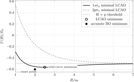
Fixed-exponent $1s$ LCAO curves including proton–proton repulsion. The open circle marks the minimum of the plotted $1s\sigma_g$ trial curve; the filled circle marks the accurate Born–Oppenheimer ground-state minimum and is not a point on an exact curve drawn here. The dashed $2p\sigma_u$ trial curve misses the exact, extremely shallow long-range polarization well.

For the fixed-exponent two-function trial space,

$$\begin{aligned} R_e^{\mathrm{LCAO}} &\simeq2.49283a_0,\\ U_e^{\mathrm{LCAO}} &\simeq-0.564831E_h. \end{aligned}$$

Relative to the dissociation limit $-0.5E_h$, this gives

$$D_e^{\mathrm{LCAO}} = 0.064831E_h \simeq1.764\,\mathrm{eV}.$$

Accurate clamped-nuclei calculations instead give approximately

$$R_e=1.99719332a_0 =1.05687\,\text{\AA},$$ $$\begin{aligned} U_e&=-0.6026346191E_h,\\ D_e&=0.1026346191E_h,\\ &\simeq2.793\,\mathrm{eV}. \end{aligned}$$

The minimal basis therefore recovers only about $63\%$ of the accurate Born–Oppenheimer well depth and overestimates the equilibrium distance by about $25\%$. This is a useful warning: obtaining the right bonding story does not imply spectroscopic accuracy.

Well depth is not dissociation from the lowest rovibrational level

$D_e$ is the depth from the potential minimum to the separated-fragment asymptote. A molecule in its lowest vibrational state has positive zero-point energy above that minimum, and finite proton masses introduce additional nonadiabatic and relativistic corrections. The dissociation energy from the rovibrational ground state, $D_0$, is therefore smaller than $D_e$. Comparisons with experiment must specify isotope, rotational state, energy zero, and which corrections are included.

Force and equilibrium

For a normalized exact electronic eigenstate at fixed $R$, the Hellmann–Feynman theorem gives

$$\frac{dU_n}{dR} = \left\langle\psi_n\left| \frac{\partial\hat h_e}{\partial R} \right|\psi_n\right\rangle -\frac{1}{R^2}.$$

Equilibrium satisfies $dU/dR=0$: the electronic force balances proton–proton repulsion. In a geometry-dependent finite basis, differentiating a variational energy also produces Pulay terms because the basis functions move with the nuclei. Omitting those terms generally gives an inconsistent force even if the energy is variational.

Why H₂⁺ Is a Two-State System

H₂⁺ realizes the abstract two-state Hamiltonian in a spatially transparent way.

Two-state language	H₂⁺ realization
localized basis	electron near nucleus $A$ or $B$
symmetry eigenbasis	$
coupling	half the gerade–ungerade splitting
detuning	asymmetry between the two centers
coherent oscillation	transfer between localized alternatives
avoided crossing	level repulsion when biased localized states mix

For identical nuclei there is no site-energy bias. If an external field or a heteronuclear substitution makes the localized alternatives inequivalent, the projected Hamiltonian takes the generic form

$$\hat H_{\mathrm{eff}} = \bar\epsilon\,\mathbf 1 +\frac{\Delta}{2}\sigma_z -\tau\sigma_x.$$

Its level separation is

$$\Omega_E=\sqrt{\Delta^2+4\tau^2}.$$

This is the same algebra developed for Two-State Hamiltonians and the Tight-Binding Dimer. H₂⁺ supplies microscopic Coulomb matrix elements and a geometry-dependent coupling instead of taking $\Delta$ and $\tau$ as phenomenological constants.

Limits of the analogy

The two-state reduction is controlled only when the selected $g/u$ pair is well separated from other electronic states and the nuclear geometry is treated consistently. At short distance, many united-atom orbitals are relevant to localized descriptions. During fast nuclear motion, derivative couplings can mix electronic channels. In a strong field, polarization and ionization require a larger basis or continuum states. A two-by-two Hamiltonian is a projection, not the full molecule.

Nor are $\phi_A$ and $\phi_B$ themselves an orthonormal qubit basis at finite $R$. The localized $|L\rangle,|R\rangle$ states above are constructed from orthonormal exact parity eigenstates. Using raw overlapping atomic orbitals as if they were orthogonal changes transition probabilities and matrix elements.

Limiting Cases and Diagnostic Checks

Separated fragments

As $R\to\infty$,

$$S,J,K\to0, \qquad U_g,U_u\to-\frac12E_h.$$

The splitting vanishes, and any normalized linear combination of the degenerate $g/u$ pair is also an eigenstate in the limit. The localized alternatives then correlate with H $+$ p, with the electron on either identical center. At large but finite $R$, exchange produces an exponentially small parity splitting while polarization contributes a common algebraic attraction.

United atom

As $R\to0$, the electronic Coulomb potential approaches that of He⁺,

$$-\frac1{r_A}-\frac1{r_B} \longrightarrow -\frac2r.$$

The exact ground electronic eigenvalue tends to $-2E_h$. Nevertheless,

$$U_g(R)=\epsilon_g(R)+\frac1R\longrightarrow+\infty$$

because the nuclear repulsion diverges. The exact gerade state correlates with the He⁺ $1s$ orbital, while the lowest ungerade $\sigma$ state correlates with a $2p_z$-like united-atom orbital.

The fixed-exponent minimal basis cannot reproduce this limit. As the centers merge, $\phi_A$ and $\phi_B$ become linearly dependent, $S\to1$, and the ungerade normalization contains $1-S\to0$. The limiting difference $\phi_A-\phi_B$ can encode a derivative-like $p_z$ shape only after careful rescaling, while the fixed exponent remains wrong for charge $Z=2$.

Variational ordering

Within each symmetry sector, the lowest Ritz value is an upper bound to the corresponding exact fixed-$R$ electronic eigenvalue. Adding $1/R$ preserves the inequality at that same geometry. It does not imply that an approximate equilibrium distance bounds the exact $R_e$, because minimizers of two different functions need not be ordered.

The exact nondegenerate ground state of a real scalar Schrödinger operator can be chosen nodeless. In homonuclear H₂⁺ it is consequently the even $1s\sigma_g$ state. A computed odd ground state or a lower nodal trial state is a diagnostic of a sign, normalization, or symmetry error.

What H₂⁺ Teaches

H₂⁺ establishes several durable lessons:

• a one-electron wavefunction can be delocalized over several nuclei without invoking electron–electron correlation;
• bonding and antibonding combinations arise from symmetry plus variational mixing;
• overlap is a metric, not merely a pictorial measure of orbital contact;
• a potential curve requires both the electronic energy and nuclear repulsion;
• qualitative LCAO physics can be right while equilibrium properties remain quantitatively poor;
• tunneling language refers to superpositions and dynamics, not motion inside a stationary parity eigenstate;
• molecular labels acquire meaning through symmetry and correlation limits, not through pictures alone.

It does not show that every covalent bond is simply one electron tunneling between atoms. Multi-electron molecules require antisymmetry, spin coupling, electron correlation, and often several configurations. Valence Bond Theory and Molecular Orbitals provide complementary many-electron languages; neither is licensed by H₂⁺ to ignore the full many-electron state. Hydrogen Molecule takes the next step explicitly and shows why simply doubly occupying the H₂⁺ bonding orbital fails at neutral dissociation. Chemical Bonding places both examples inside the wider covalent, ionic, metallic, and weak-interaction diagnostic framework.

Common Mistakes

• Calling $\epsilon(R)$ the molecular potential. The nuclear repulsion $1/R$ must be added before discussing equilibrium or vibrational motion.
• Using $1/\sqrt2$ normalization at finite separation. The correct denominators contain $1\pm S$.
• Diagonalizing $\mathbf H$ while ignoring $\mathbf S$. Atom-centered functions form a nonorthogonal basis, so the secular equation is generalized.
• Treating $H_{01}$ alone as an observable hopping energy. The inferred coupling depends on orthogonalization; the eigenvalue splitting does not.
• Assuming an antibonding label forbids every bound level. The exact $2p\sigma_u$ curve has a tiny long-range polarization well.
• Comparing $D_e$ directly with a measured $D_0$. Zero-point, finite-mass, relativistic, and radiative effects must be matched consistently.
• Interpreting a parity eigenstate as a localized electron in motion. Stationary $g/u$ densities do not oscillate.
• Taking the minimal LCAO curve as exact because the molecule has one electron. The electronic problem is one-body, but a two-function trial space is still severely incomplete.

Exercises

1. Generalized secular equation

Starting from $\psi=c_A\phi_A+c_B\phi_B$, derive the two secular energies for a homonuclear two-center basis with overlap $S$. Verify the normalization constants of the corresponding eigenvectors.

Solution

Stationarity gives

$$\det(\mathbf H-\epsilon\mathbf S)=0.$$

With equal diagonal elements,

$$\begin{vmatrix} H_{00}-\epsilon&H_{01}-\epsilon S\\ H_{01}-\epsilon S&H_{00}-\epsilon \end{vmatrix}=0.$$

Therefore

$$(H_{00}-\epsilon)^2 -(H_{01}-\epsilon S)^2=0,$$

which factors into even and odd equations. The roots are

$$\epsilon_g=\frac{H_{00}+H_{01}}{1+S}, \qquad \epsilon_u=\frac{H_{00}-H_{01}}{1-S}.$$

The coefficient vectors are proportional to $(1,1)^T$ and $(1,-1)^T$. Their metric norms are

$$(1,\pm1) \begin{pmatrix}1&S\\S&1\end{pmatrix} \begin{pmatrix}1\\\pm1\end{pmatrix} =2(1\pm S),$$

which yields the stated factors $[2(1\pm S)]^{-1/2}$.

2. Overlap checks

For

$$S(R)=e^{-R}\left(1+R+\frac{R^2}{3}\right),$$

show that $S(0)=1$, $S(\infty)=0$, and $S'(R)<0$ for $R>0$. Explain why these checks matter physically.

Solution

The endpoint values follow directly. Differentiating gives

$$S'(R) =e^{-R} \left[ 1+\frac{2R}{3} -1-R-\frac{R^2}{3} \right],$$

so

$$S'(R) =-\frac{R(1+R)}{3}e^{-R}<0$$

for $R>0$. Coincident normalized functions must have unit overlap; infinitely separated localized functions must have zero overlap; and increasing separation should reduce their overlap monotonically. Failure of any check signals an integration or convention error.

3. Energies at two bohr

Using the analytic $S$, $J$, and $K$ expressions, reproduce the LCAO values of $U_g$ and $U_u$ at $R=2a_0$. Which state is below the separated-fragment threshold?

Solution

At $R=2$,

$$S=e^{-2}\left(1+2+\frac43\right) =0.5864528940,$$ $$J=-\frac12+\frac32e^{-4} =-0.4725265417,$$ $$K=-3e^{-2} =-0.4060058497.$$

Substitution gives

$$\begin{aligned} U_g(2) &=\frac{J+K}{1+S}\\ &=-0.5537714953E_h, \end{aligned}$$

and

$$\begin{aligned} U_u(2) &=\frac{J-K}{1-S}\\ &=-0.1608539656E_h. \end{aligned}$$

Only the gerade trial energy lies below $-0.5E_h$ at this separation.

4. Large-separation splitting

Show from the secular energies that the $g/u$ splitting vanishes as $R\to\infty$. Why does this make a localized electronic state possible in the strict limit?

Solution

Because $S\to0$, $J\to0$, and $K\to0$, one has

$$H_{00}\to-\frac12, \qquad H_{01}\to0.$$

Thus

$$\epsilon_g,\epsilon_u\to-\frac12, \qquad \epsilon_u-\epsilon_g\to0.$$

For exact degeneracy, every linear combination of $|g\rangle$ and $|u\rangle$ is an eigenstate with the same energy. In particular, $(|g\rangle\pm|u\rangle)/\sqrt2$ can localize on opposite centers. At any finite separation the splitting is nonzero, so the localized combinations are not stationary.

5. Coherent transfer

An ideal two-state H₂⁺ model has $\epsilon_u-\epsilon_g=0.020E_h$. Find the first complete transfer time from one localized state to the other. Use $\hbar/E_h=2.418884\times10^{-17}\,\mathrm{s}$.

Solution

The first complete transfer occurs at

$$t_{L\to R} =\frac{\pi\hbar}{\epsilon_u-\epsilon_g}.$$

Therefore

$$\begin{aligned} t_{L\to R} &=\frac{\pi}{0.020} \left(2.418884\times10^{-17}\,\mathrm{s}\right)\\ &\simeq3.80\times10^{-15}\,\mathrm{s}. \end{aligned}$$

This is about $3.80\,\mathrm{fs}$. The result describes coherent electronic evolution at fixed $R$; it is not automatically the transfer time in a vibrating or decohering molecule.

6. Quantifying the minimal-basis error

Using the minima quoted above, calculate the percentage error in $R_e$, the fraction of the accurate $D_e$ recovered by minimal LCAO, and the variational energy error at the respective minima.

Solution

The bond-length error is

$$\frac{2.492827-1.997193}{1.997193}\times100\% \simeq24.8\%.$$

The recovered fraction of the well depth is

$$\frac{0.064831}{0.102635} \simeq0.632,$$

or about $63.2\%$. Comparing the minimum energies gives

$$\begin{aligned} U_e^{\mathrm{LCAO}}-U_e^{\mathrm{exact}} &\simeq0.037804E_h,\\ &\simeq1.029\,\mathrm{eV}. \end{aligned}$$

The positive energy difference is consistent with the variational principle. Because the two values occur at different geometries, it is a comparison of optimized approximate and exact curves, not the fixed-geometry variational error.

7. United-atom correlations

Explain why the exact $1s\sigma_g$ and $2p\sigma_u$ states correlate with He⁺ $1s$ and $2p_z$ orbitals as $R\to0$. Why does the total energy still diverge?

Solution

When the protons coincide, their charges add and the electronic potential becomes $-2/r$. The lowest nodeless even state therefore approaches the He⁺ $1s$ orbital. The lowest odd state along the internuclear axis must change sign through the midpoint and has $m=0$, matching the symmetry of a $2p_z$ orbital.

The electronic energies remain finite in this united-atom limit, but the two distinct protons still contribute

$$V_{NN}=\frac1R.$$

Consequently the molecular Born–Oppenheimer potential diverges to $+\infty$ as $R\to0$.

8. Distinguishing Dₑ and D₀

Suppose a calculation gives a Born–Oppenheimer well depth $D_e$ and a nuclear ground-state energy $E_{v=0}$ measured upward from the potential minimum. Ignoring all other corrections, express $D_0$ in terms of these quantities. List three reasons why a precision experimental comparison needs more information.

Solution

With the stated energy zero,

$$D_0=D_e-E_{v=0}.$$

A precision comparison also needs, among other items, the isotopologue and nuclear masses, the initial rotational quantum number, nonadiabatic corrections, relativistic and radiative corrections, and a consistent separated-fragment energy. Quoting only a clamped-nuclei $D_e$ does not specify the measured dissociation threshold.

References

1. M. Born and R. Oppenheimer, “Zur Quantentheorie der Molekeln,” Annalen der Physik 389, 457–484 (1927), doi:10.1002/andp.19273892002.
2. Ø. Burrau, “Berechnung des Energiewertes des Wasserstoffmolekel-Ions (H₂⁺) im Normalzustand,” Kongelige Danske Videnskabernes Selskab, Mathematisk-fysiske Meddelelser 7(14), 1–18 (1927).
3. C. Y. Chao, “The Problem of the Ionized Hydrogen Molecule,” Proceedings of the National Academy of Sciences 15, 558–565 (1929), doi:10.1073/pnas.15.7.558.
4. D. R. Bates, K. Ledsham, and A. L. Stewart, “Wave Functions of the Hydrogen Molecular Ion,” Philosophical Transactions of the Royal Society A 246, 215–240 (1953), doi:10.1098/rsta.1953.0014.
5. J. M. Peek, “Eigenparameters for the $1s\sigma_g$ and $2p\sigma_u$ Orbitals of H₂⁺,” Journal of Chemical Physics 43, 3004–3006 (1965), doi:10.1063/1.1697265.
6. J. M. Peek, “Discrete Vibrational States Due Only to Long-Range Forces: $^2\Sigma_u^+(2p\sigma_u)$ State of H₂⁺,” Journal of Chemical Physics 50, 4595–4601 (1969), doi:10.1063/1.1670939.
7. M. M. Madsen and J. M. Peek, “Eigenparameters for the Lowest Twenty Electronic States of the Hydrogen Molecule Ion,” Atomic Data and Nuclear Data Tables 2, 171–204 (1971), doi:10.1016/S0092-640X(70)80008-0.
8. C. L. Beckel, B. D. Hansen III, and J. M. Peek, “Theoretical Study of H₂⁺ Ground Electronic State Spectroscopic Properties,” Journal of Chemical Physics 53, 3681–3690 (1970).
9. C. A. Leach and R. E. Moss, “Spectroscopy and Quantum Mechanics of the Hydrogen Molecular Cation: A Test of Molecular Quantum Mechanics,” Annual Review of Physical Chemistry 46, 55–82 (1995), doi:10.1146/annurev.pc.46.100195.000415.
10. Y. P. Zhang et al., “Dissociation Energies of Molecular Hydrogen and the Hydrogen Molecular Ion,” Physical Review Letters 92, 203003 (2004), doi:10.1103/PhysRevLett.92.203003.
11. K. Ruedenberg, “Why Does Electron Sharing Lead to Covalent Bonding? A Variational Analysis,” Journal of Computational Chemistry 28, 390–404 (2007), doi:10.1002/jcc.20553.
12. F. M. Fernández and J. Garcia, “Highly Accurate Potential Energy Curves for the Hydrogen Molecular Ion,” ChemistrySelect 6, 9527–9534 (2021), doi:10.1002/slct.202102509.
13. P. W. Atkins and R. S. Friedman, Molecular Quantum Mechanics, 5th ed. (Oxford University Press, 2011), Chapters 8–9.
14. I. N. Levine, Quantum Chemistry, 7th ed. (Pearson, 2014), Chapters 13–14.
15. L. D. Landau and E. M. Lifshitz, Quantum Mechanics: Non-Relativistic Theory, 3rd ed. (Pergamon, 1977), Section 81.