Chemical Bonding

A chemical bond is a durable pattern of quantum-mechanical stabilization and structure that makes it useful to regard atoms or fragments as one aggregate. The word compresses several kinds of evidence: a bound or metastable state, an equilibrium geometry, a dissociation energy, characteristic forces and spectra, and reproducible changes in electronic density or response.

No universal bond potential is added to the molecular Hamiltonian. In the standard nonrelativistic model, electrons and nuclei have kinetic energy and charged particles interact through Coulomb terms. Bonding emerges after the many-particle state adjusts subject to symmetry, antisymmetry, boundary conditions, and the chosen environment.

This immediately gives two guardrails:

• the existence and strength of binding are total-energy or free-energy questions;
• orbital pictures, Lewis structures, atomic charges, bond orders, bond paths, and energy components are analyses of a state, not interchangeable observables.

The distinction does not make chemical language arbitrary. A good bonding description is constrained by converged calculations, spectroscopy, thermochemistry, scattering, structure, response, and limiting cases. It does mean that every numerical bond claim needs an operational definition.

Canonical Scope

This page is the canonical home for:

• the operational meaning of a chemical bond in quantum mechanics;
• the distinction among binding, bond strength, bond multiplicity, and bond character;
• broad covalent, ionic, metallic, hydrogen-bonded, induction-bound, and dispersion-bound limits;
• the roles of electrostatics, antisymmetry, orbital relaxation, and electron correlation;
• the hierarchy from observables to representation-dependent bonding analyses;
• careful use of bond orders, density differences, atomic charges, bond paths, and energy decompositions;
• common misconceptions and a reproducible workflow for bonding claims.

Potential Energy Surfaces owns molecular energy landscapes, stationary points, thresholds, and nuclear motion. Molecular Orbitals owns LCAO equations, symmetry labels, occupations, and frontier-orbital language. Valence Bond Theory owns localized spin-coupled structures and resonance. Hydrogen Molecule owns the canonical two-electron covalent derivation. Electronic Structure Overview owns the basis, method, state, and error-budget map used to test whether a bonding interpretation is numerically defensible. This page compares the physical questions those representations can and cannot answer.

What Is a Bond in Quantum Mechanics?

Start from a dissociation channel

For fixed nuclear geometry $\mathbf R$, let an electronic state satisfy

$$\hat H_e(\mathbf R) |\Psi_k(\mathbf R)\rangle = E_k(\mathbf R) |\Psi_k(\mathbf R)\rangle.$$

If the electronic convention excludes internuclear repulsion, the corresponding Born–Oppenheimer surface is

$$U_k(\mathbf R) = E_k(\mathbf R) +V_{NN}(\mathbf R).$$

Choose a physically allowed fragment channel $A+B$ with the same conserved total charge and all required spin and symmetry labels. Its asymptotic threshold is

$$E_{\mathrm{th}}^{A+B} = \lim_{R\to\infty}U_k(R),$$

provided that this adiabatic surface correlates with the stated fragments. For a diatomic minimum at $R_e$, the electronic well depth is

$$D_e = E_{\mathrm{th}}^{A+B} -U_k(R_e).$$

A positive $D_e$ says that the bottom of the chosen electronic well lies below that threshold. It does not yet prove that nuclear motion has a bound level. The nuclear Hamiltonian on the surface,

$$\hat H_{\mathrm{nuc}} = \hat T_{\mathrm{nuc}} +U_k(\mathbf R),$$

must support at least one normalizable eigenstate with energy below every open dissociation channel. If its lowest rovibrational energy is $E_{v=0}$, then

$$D_0 = E_{\mathrm{th}}^{A+B} -E_{v=0}, \qquad D_0<D_e$$

for an ordinary bound well with positive zero-point energy.

A local minimum above a lower threshold can instead describe a metastable resonance. Its physical characterization requires a lifetime or width, not merely a geometry. At finite temperature, in solution, or under pressure, the relevant stability criterion may be a Helmholtz or Gibbs free-energy difference rather than an isolated-molecule energy.

Forces and equilibrium

For an exact differentiable electronic eigenstate, the Hellmann–Feynman relation gives

$$\frac{\partial E_k}{\partial R_A} = \left\langle\Psi_k\left| \frac{\partial\hat H_e}{\partial R_A} \right|\Psi_k\right\rangle.$$

The force on nucleus $A$ is

$$\mathbf F_A = -\nabla_{\mathbf R_A}U_k.$$

At an unconstrained equilibrium geometry the internal forces vanish, and the internal-coordinate Hessian is positive for a true minimum. Vanishing net force does not mean that attractive and repulsive contributions have disappeared. It means that their total derivative balances at that geometry.

Approximate wavefunctions that are not fully stationary with respect to their parameters require response terms in analytic gradients. A visually plausible density is not a substitute for a converged force calculation.

Evidence and interpretation

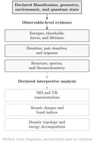
Bonding claims should be anchored in observable-level consequences of a declared Hamiltonian and state. Orbitals, charges, bond indices, and energy components are useful lower-level interpretations whose method and partition must be reported.

Three questions are often conflated:

Question	Evidence and qualification
Does an aggregate exist?	Use a bound level, resonance, or thermodynamically stable phase; state the channel, environment, and lifetime.
How hard is it to separate?	Specify $D_e$, $D_0$, a bond-dissociation enthalpy, or a free energy; these can use different products.
Where and what kind is the bond?	Combine densities, spectra, response, orbitals, structures, and indices; no single analysis is universal.

IUPAC definitions deliberately include a pragmatic stability criterion: an aggregate must be sufficiently stable to be treated as an independent species in the chemical context. Quantum mechanics sharpens that idea through thresholds, lifetimes, and free energies, but it does not create one context-free numerical boundary between “bonded” and “not bonded.”

There is no universal bond operator

An observable in quantum mechanics is represented by an operator or measurement protocol. There is no state-independent Hermitian operator $\hat B_{AB}$ whose eigenvalues count chemical bonds between every possible pair of atoms in every molecule, crystal, excited state, solvent, and reaction.

Bond graphs are therefore a physically disciplined coarse-graining. They are successful because many electronic and nuclear states display robust locality, energy gaps, recurring valences, and transferable response patterns. The graph can remain stable under small changes in method even though its detailed orbital or density partition is not unique.

Covalent Bonding

Coherent two-center mixing

Let normalized atom-centered orbitals $a(\mathbf r)$ and $b(\mathbf r)$ have real overlap

$$S=\langle a|b\rangle.$$

The normalized bonding combination is

$$g(\mathbf r) = \frac{a(\mathbf r)+b(\mathbf r)} {\sqrt{2(1+S)}}.$$

Its one-electron density is

$$\rho_g(\mathbf r) = \frac{ |a|^2+|b|^2 +2\operatorname{Re}(a^*b) }{2(1+S)}.$$

The interference term can increase density between the centers when the orbital phases agree there. The antibonding combination reverses its sign and introduces an additional node:

$$u(\mathbf r) = \frac{a(\mathbf r)-b(\mathbf r)} {\sqrt{2(1-S)}}.$$

This algebra explains why phase coherence matters, but it is not by itself a proof of binding. The normalization changes with $S$; orbitals relax when atoms approach; electron–nuclear attraction, kinetic energy, electron–electron repulsion, and internuclear repulsion all change. Only the total molecular energy relative to a declared fragment limit decides stability.

H₂⁺ Ion evaluates these statements for the exact one-electron two-center Hamiltonian and its minimal LCAO approximation.

Spin coupling and electron pairs

For two electrons in localized orbitals, a normalized covalent spatial function is

$$\Phi_{\mathrm{cov}}^+ = \frac{ a(1)b(2)+b(1)a(2) }{ \sqrt{2(1+S^2)} }.$$

It is symmetric under electron exchange and therefore pairs with the antisymmetric spin singlet. The corresponding antisymmetric spatial combination pairs with a triplet.

This exchange-symmetry constraint is essential, but “exchange” is not an additional microscopic force. The Hamiltonian remains Coulombic. Antisymmetry changes the admissible state, its nodes, kinetic energy, pair density, and Coulomb expectation values.

Hydrogen Molecule derives the direct and exchange matrix elements, compares Heitler–London and molecular-orbital states, and shows why a restricted one-determinant description fails at neutral dissociation.

Localized and delocalized descriptions

A covalent bond can be represented by:

• localized spin-coupled valence-bond structures;
• occupied delocalized molecular orbitals;
• localized orbitals obtained by unitary rotations of occupied orbitals;
• reduced density matrices, pair densities, or correlated geminals.

Complete MO and VB expansions describe the same antisymmetric Hilbert space. Their practical differences come from truncation and optimization. A compact localized expansion may expose fragment spin coupling; a compact delocalized determinant may expose symmetry and shell filling. Neither representation has exclusive ownership of the exact state.

Covalency also extends beyond a single two-center, two-electron pair. Three-center bonds, electron-deficient clusters, aromatic delocalization, multiple bonds, and multicenter spin coupling require a larger orbital and configuration space. A Lewis structure can be an excellent summary without being a literal assignment of distinguishable electrons.

Polar covalency

Homonuclear and purely ionic limits are endpoints, not exhaustive categories. Unequal orbital energies and environment-dependent polarization usually mix neutral and charge-transfer structures. A polar covalent bond may have:

• appreciable density sharing and orbital mixing;
• a nonzero dipole moment;
• unequal atomic populations in a declared partition;
• both covalent and ionic amplitudes in a VB expansion.

The percentage labels depend on the basis and population scheme. Observable dipole moments and dissociation products constrain the interpretation more directly.

Ionic Bonding

Charge-transfer energetics

Consider a donor $A$ and acceptor $B$. At large separation, the energy cost of the ionic channel $A^+B^-$ relative to neutral fragments is approximately

$$\Delta_\infty = I_A-\mathcal A_B,$$

where $I_A$ is the ionization energy of $A$ and $\mathcal A_B$ is the electron affinity of $B$. At finite separation, define the point-charge contribution

$$\Delta_C(R) = -\frac{e^2}{4\pi\epsilon_0R}.$$

Let

$$\Delta_{IN}(R) \equiv E_I(R)-E_N(R).$$

Then

$$\begin{aligned} \Delta_{IN}(R) \simeq{}& \Delta_\infty\\ &+\Delta_C(R)\\ &+\Delta E_{\mathrm{pol}}(R)\\ &+\Delta E_{\mathrm{overlap}}(R) +\cdots . \end{aligned}$$

The attractive Coulomb term can make the ionic channel competitive, while polarization, finite charge distributions, orbital overlap, short-range antisymmetry, and correlation modify the point-charge picture.

Neutral–ionic mixing

In an orthonormal diabatic basis $\{|N\rangle,|I\rangle\}$, write

$$\mathbf H_d(R) = \begin{pmatrix} E_N(R)&V(R)\\ V(R)&E_I(R) \end{pmatrix}.$$

Define

$$\bar E=\frac{E_N+E_I}{2}, \qquad \Delta=E_I-E_N.$$

The adiabatic energies are

$$E_\pm = \bar E \pm \frac12\sqrt{\Delta^2+4V^2}.$$

For the lower state, one convenient phase convention gives the ionic weight

$$w_I = \frac12 \left( 1-\frac{\Delta}{\sqrt{\Delta^2+4V^2}} \right).$$

When $\Delta\gg|V|$, the state is mostly neutral; when $-\Delta\gg|V|$, it is mostly ionic; at a diabatic crossing it is an equal mixture and the adiabatic gap is $2|V|$. The numerical value of $w_I$ is not unique if the diabatic structures are changed or are nonorthogonal, but the avoided crossing, adiabatic energies, dipole, and response are physical.

Ions in solids and environments

An ionic crystal is not a collection of isolated gas-phase ion pairs. Its stability includes:

• the collective Madelung electrostatic energy of the lattice;
• short-range overlap and antisymmetry;
• ionic polarization and many-body induction;
• zero-point lattice motion and thermal phonons;
• possible covalent mixing, defects, surfaces, and charge transfer;
• the energy required to create the ions from neutral reference states.

Formal oxidation states are exact bookkeeping rules within a chosen chemical convention. Partial atomic charges are partition-dependent. Neither should be confused with measuring a point charge located on an atom.

Solvation can reverse gas-phase preferences because ionic and neutral channels receive different polarization free energies. A statement such as “this bond is ionic” is incomplete without the state, geometry, phase, and diagnostic.

Metallic Bonding Preview

Metallic cohesion is an extended many-electron problem. If one orbital per atom is coupled along a periodic one-dimensional chain, the nearest-neighbor tight-binding model gives

$$\varepsilon(k) = \varepsilon_0-2t\cos(ka).$$

As the number of atoms grows, discrete bonding and antibonding levels become a band. A partially filled band has low-energy particle–hole excitations near its Fermi surface and can carry current when scattering and interactions are treated appropriately.

The Tight-Binding Model owns this lattice reduction and its validity conditions. Several cautions matter for bonding:

• a delocalized Bloch orbital is not a classical electron trajectory through the lattice;
• a completely filled band can be strongly cohesive and electrically insulating;
• conductivity is not a definition of bond strength;
• localized Wannier functions can represent the same occupied band subspace;
• the total cohesive energy also contains ion–ion terms, electron interactions, screening, correlation, and double-counting corrections appropriate to the method.

The phrase “electron sea” is a useful limiting image for simple $s$-band metals, not a universal microscopic description. Transition metals, narrow bands, magnetism, Mott physics, and directional orbital hybridization require more structure.

Hydrogen Bonding and Weak Interactions

Hydrogen bonds require evidence

A hydrogen bond is an attractive interaction in which hydrogen bound to an atom or group $X$ interacts with an atom or group $Y$, with experimental or theoretical evidence that a specific association has formed. Modern usage is broader than the mnemonic “H attached to N, O, or F,” although those donors and acceptors are common.

Useful evidence can include:

• an interaction energy or free energy relative to separated partners;
• donor–acceptor geometry and a reproducible distance contraction;
• changes in the $X$–H stretching frequency and intensity;
• NMR, rotational, vibrational, or electronic spectroscopic signatures;
• isotope effects;
• systematic density, orbital, or energy-decomposition changes;
• consistency across a family of structures and competing conformers.

No universal distance cutoff proves a hydrogen bond. A short contact can be imposed by sterics or a crystal lattice, while a real weak interaction can be longer than a tabulated sum of radii.

An interaction is a balance, not one mechanism

For two fragments, symmetry-adapted perturbation theory organizes the interaction energy schematically as

$$\begin{aligned} E_{\mathrm{int}} ={}&E_{\mathrm{elst}}+E_{\mathrm{exch}}\\ &+E_{\mathrm{ind}}+E_{\mathrm{disp}}\\ &+E_{\mathrm{exch\text{-}ind}}\\ &+E_{\mathrm{exch\text{-}disp}} +\cdots . \end{aligned}$$

The terms have clear definitions only within the stated SAPT order, monomer method, basis, and partition. Other energy-decomposition analyses divide the same total differently.

Mechanism	Origin and qualification
electrostatics	Permanent charge distributions and multipoles interact; penetration matters when densities overlap.
induction	One fragment polarizes another; the assigned term depends on the fragment response space.
dispersion	Correlated quantum fluctuations attract; ordinary single-determinant Hartree–Fock misses the long-range term.
exchange overlap	Antisymmetrization changes overlapping fragment states; this is not a new pair potential and usually decays exponentially.

For isotropic ground-state fragments in the nonretarded long-range limit,

$$E_{\mathrm{disp}}(R) \sim -\frac{C_6}{R^6}.$$

In Hartree atomic units, the Casimir–Polder representation is

$$C_6 = \frac3\pi \int_0^\infty \alpha_A(i\omega) \alpha_B(i\omega) \,d\omega,$$

where $\alpha_A$ and $\alpha_B$ are dynamic dipole polarizabilities evaluated at imaginary frequency. At asymptotically larger separations, electromagnetic retardation changes the power law; ordinary molecular separations are usually in the nonretarded regime.

Hydrogen bonds, halogen bonds, $\pi$ stacking, ion–molecule complexes, and dispersion-bound dimers all combine several of these mechanisms. Naming the interaction identifies a recurring geometry and chemical pattern; it does not isolate one term of the Hamiltonian.

Cooperativity and many-body effects

Pairwise additivity is an approximation. A third molecule can polarize both members of a pair, alter charge-transfer amplitudes, change exchange overlap, and contribute three-body dispersion. Hydrogen-bond networks can therefore be cooperative or anticooperative depending on geometry and electronic response.

In condensed phases, entropy and solvent reorganization can be as important as the isolated interaction energy. A deep gas-phase minimum need not imply a favorable solution-phase association free energy.

Exchange, Correlation, and Electrostatics

One density is not enough for every energy

Let the spin-summed pair density $P(\mathbf r,\mathbf r')$ be normalized by

$$\int d^3r\,d^3r'\, P(\mathbf r,\mathbf r') = N(N-1).$$

The exact electron–electron interaction energy is

$$E_{ee} = \frac{e^2}{8\pi\epsilon_0} \int \frac{ P(\mathbf r,\mathbf r') }{ |\mathbf r-\mathbf r'| } \,d^3r\,d^3r'.$$

The one-electron density $\rho(\mathbf r)$ determines many observables, but the pair density records conditional electron avoidance. A single determinant includes the exchange hole required by antisymmetry. Correlated states modify opposite-spin and same-spin pair structure beyond that determinant.

Exchange and Correlation develops the direct, exchange, pair-hole, and density-functional bookkeeping. Reduced Density Matrices provides the general subsystem language.

What “Pauli repulsion” means

When closed-shell fragments overlap, antisymmetrization forces occupied orbitals into an orthogonal many-electron state. The resulting energy increase is often called Pauli, exchange, or steric repulsion. These phrases summarize changes in kinetic and Coulomb expectation values caused by the restricted state space.

There is no additional repulsive term in the exact Coulomb Hamiltonian labeled “Pauli.” An exponential short-range potential can be a useful effective fit, but it is not a new fundamental force.

Correlation can strengthen or weaken binding

For a fixed Hamiltonian and complete one-electron basis,

$$E_{\mathrm{corr}} = E_{\mathrm{exact}}-E_{\mathrm{HF}} \leq0.$$

The correlation contribution to a binding energy is instead a difference of differences. Define

$$E_{\mathrm{corr}}(A+B) = E_{\mathrm{corr}}(A) +E_{\mathrm{corr}}(B).$$

Then

$$\Delta D_e^{\mathrm{corr}} = E_{\mathrm{corr}}(A+B) -E_{\mathrm{corr}}(AB).$$

It can be positive or negative. Correlation is essential for long-range dispersion and for symmetry-preserving dissociation of stretched H₂, but it does not follow that correlation strengthens every bond. Fragment and molecular correlation energies compete.

Hartree–Fock Approximation derives the determinant mean field and explains precisely what it includes and omits.

Total-energy partitions

For the nonrelativistic Coulomb Hamiltonian, one can write the change on assembly as

$$\Delta E = \Delta T +\Delta V_{eN} +\Delta V_{ee} +\Delta V_{NN}.$$

These expectation values are defined once the Hamiltonian, state, geometry, and fragment comparison are fixed. Their changes can be individually large and cancel strongly. Further labels such as orbital interaction, charge transfer, polarization, steric energy, covalency, and preparation energy depend on a chosen path and partition.

Energy decomposition is valuable when it answers a declared comparative question and remains stable under reasonable methodological changes. Its components should not be reported as directly measurable fractions of a bond.

Bond Order and Electron Density

Strength, stiffness, and multiplicity differ

Several quantities are informally called bond strength:

$$D_e = E_{\mathrm{fragments}} -E_{\mathrm{minimum}},$$ $$k_e = \left. \frac{d^2U}{dR^2} \right|_{R=R_e},$$

and a thermochemical bond-dissociation enthalpy for a specified homolytic or heterolytic reaction. A deep well, a large harmonic force constant, a short equilibrium distance, and a large electronic bond index often correlate within a chemical family, but none determines all the others.

Zero-point energy distinguishes $D_0$ from $D_e$. Fragment relaxation distinguishes a vertical separation from an adiabatic dissociation. Spin–orbit levels, charge states, temperature, and phase must be included when they matter.

Orbital bond order

For a chosen bonding–antibonding orbital pair, the familiar index is

$$b_{\mathrm{MO}} = \frac{ N_{\mathrm{bonding}} -N_{\mathrm{antibonding}} }{2}.$$

This is effective bookkeeping in small orbital diagrams. It is not a universal observable. The restricted $g^2$ description of H₂ has $b_{\mathrm{MO}}=1$ at every separation even though it dissociates incorrectly.

For an orthonormal atomic-orbital partition, one Wiberg-type closed-shell index has the form

$$W_{AB} = \sum_{\mu\in A} \sum_{\nu\in B} |P_{\mu\nu}|^2,$$

where $P$ is a spin-summed one-particle density matrix in the stated normalization. Mayer-type indices adapt the construction to a nonorthogonal basis through the overlap matrix $S$. Numerical factors and open-shell generalizations vary by convention.

Such indices can be excellent comparative descriptors along a reaction or within a method-consistent series. They depend on the basis, orbital partition, density matrix, and population prescription.

Density differences

A common visualization is the frozen-fragment density difference

$$\Delta\rho(\mathbf r) = \rho_{AB}(\mathbf r) -\rho_A^{\mathrm{frag}}(\mathbf r) -\rho_B^{\mathrm{frag}}(\mathbf r).$$

If the fragment densities contain the same total number of electrons as the aggregate,

$$\int\Delta\rho(\mathbf r)\,d^3r=0.$$

Positive and negative regions show redistribution, not creation and destruction of charge. The picture depends on fragment geometries, electronic states, alignment, and whether the fragment densities are frozen or relaxed.

Density accumulation between nuclei can support a covalent interpretation, but it is neither necessary nor sufficient for every bond. Polar, multicenter, charge-shift, closed-shell, and transition-metal interactions can have different signatures.

Density topology and localization

In the quantum theory of atoms in molecules, atomic basins are bounded by zero-flux surfaces of $\nabla\rho$, and a bond path passes through a rank-three, signature-minus-one critical point when that topology exists. This is a precise statement about a chosen electron density.

A bond critical point is not automatically:

• a measure of bond energy;
• proof of a conventional two-center bond;
• a unique chemical graph for every purpose;
• interchangeable with an orbital bond order.

Electron-localization functions, natural bond orbitals, localized MOs, delocalization indices, source functions, and pair-density analyses answer other questions. Agreement among independent diagnostics is stronger evidence than a single colorful isosurface.

Match the diagnostic to the question

Diagnostic	Use and limitation
dissociation or association energy	Tests stability against a specified channel, not local multiplicity in a polyatomic molecule.
force constant and spectrum	Probes local curvature and nuclear dynamics, not the asymptotic dissociation energy.
density and density difference	Shows charge distribution and redistribution, not a unique energy decomposition.
orbital or density-matrix index	Tracks multiplicity within a convention, not a basis-independent observable bond count.
interaction-energy decomposition	Compares mechanisms in one scheme, not unique measurable percentages.

Common Misconceptions

• “A bond is a force term in the Hamiltonian.” The microscopic terms are kinetic and Coulombic in the standard model; bonding is a property of the resulting state and energy landscape.
• “More density between nuclei always means a stronger bond.” Density, kinetic energy, pair structure, nuclear repulsion, and the dissociation channel must all be considered.
• “Exchange is a new attractive or repulsive force.” Exchange effects follow from antisymmetry and a chosen state or partition.
• “Correlation is the cause of every bond.” Hartree–Fock binds many molecules qualitatively, while correlation can strengthen or weaken a binding energy and is indispensable in particular limits.
• “Covalent and ionic are mutually exclusive exact labels.” Real eigenstates commonly mix neutral and charge-transfer structures.
• “Atomic charges are observables.” Molecular multipole moments are observable; assigning that density to atoms requires a partition.
• “A bond order is the number of bonds measured by quantum mechanics.” It is an index tied to a representation and convention.
• “Hydrogen bonding is purely electrostatic.” Electrostatics is important, but exchange, induction, dispersion, and sometimes appreciable charge-transfer-like response coexist.
• “Metallic bonding means free classical electrons.” Bloch states, screening, band filling, correlations, and lattice dynamics replace that literal picture.
• “A local minimum proves a stable molecule.” Zero-point motion or a lower open channel can turn it into an unbound state or resonance.
• “A shorter bond must be stronger.” Relativistic effects, sterics, charge, coordination, electronic state, and the selected dissociation products can reverse simple trends.
• “One energy decomposition reveals the true percentages.” Decomposition components depend on fragments, paths, basis sets, and definitions even when the total energy agrees.

A Defensible Bonding Workflow

1. State the physical system. Give composition, charge, spin, electronic state, geometry, phase, temperature, fields, and environment.
2. Declare the Hamiltonian and approximation. Identify Born–Oppenheimer, relativistic, pseudopotential, solvent, periodic, and correlation assumptions.
3. Specify the comparison. Name the dissociation or association channel and whether energies are vertical, adiabatic, zero-point corrected, enthalpic, or free energetic.
4. Converge observable-level quantities. Test basis, correlation treatment, integration grids, finite-size effects, and geometry.
5. Check more than one signature. Combine energies or forces with density, spectroscopy, response, and limiting behavior.
6. Choose an analysis for a question. Use MO, VB, population, topology, localization, or energy decomposition because it answers something specific.
7. Probe representation sensitivity. Vary orbitals, fragment definitions, basis, or partition where the diagnostic permits it.
8. Report uncertainty and scope. Separate numerical error, model error, environmental effects, and interpretive convention.

Finite atom-centered bases create an additional hazard for weak binding: the dimer can borrow basis functions from both fragments and appear artificially overbound. Counterpoise calculations and systematic basis convergence help diagnose this basis-set superposition error, but neither replaces correlation and geometry convergence.

Exercises

1. Electronic well depth versus nuclear binding

A diatomic Born–Oppenheimer surface has its minimum $0.180\,\mathrm{eV}$ below the lowest dissociation threshold. A harmonic calculation estimates the vibrational zero-point energy as $0.125\,\mathrm{eV}$ above the minimum. Find $D_e$ and the harmonic estimate of $D_0$. Would a zero-point estimate of $0.195\,\mathrm{eV}$ support a bound ground vibrational level?

Solution

The electronic well depth is

$$D_e=0.180\,\mathrm{eV}.$$

The dissociation energy from the lowest vibrational level is

$$\begin{aligned} D_0 &=D_e-E_{\mathrm{ZPE}}\\ &=0.180-0.125\\ &=0.055\,\mathrm{eV}. \end{aligned}$$

Within the harmonic estimate, the lowest level lies below threshold and is bound. If $E_{\mathrm{ZPE}}=0.195\,\mathrm{eV}$, the estimate places that level $0.015\,\mathrm{eV}$ above threshold, so it does not support a bound level. The full anharmonic nuclear Schrödinger equation is needed for a definitive conclusion near threshold.

2. Neutral–ionic avoided crossing

Take the neutral diabatic energy as zero, the ionic diabatic energy as $\Delta=4.0\,\mathrm{eV}$, and the coupling as $V=1.0\,\mathrm{eV}$. Find the lower adiabatic energy relative to the neutral state and its ionic weight. What happens when $\Delta=0$?

Solution

With $E_N=0$ and $E_I=\Delta$,

$$E_- = \frac{\Delta}{2} -\frac12\sqrt{\Delta^2+4V^2}.$$

Therefore

$$\begin{aligned} E_- &=2-\frac12\sqrt{20}\\ &\simeq-0.236\,\mathrm{eV}. \end{aligned}$$

The ionic weight is

$$\begin{aligned} w_I &=\frac12 \left(1-\frac4{\sqrt{20}}\right)\\ &\simeq0.0528. \end{aligned}$$

Thus a state that is mostly neutral is stabilized by ionic mixing. At $\Delta=0$, both adiabatic states are equal-magnitude neutral–ionic mixtures and their gap is $2|V|=2.0\,\mathrm{eV}$.

3. Normalize the bonding density

For real normalized functions $a$ and $b$ with overlap $S$, verify that

$$g=\frac{a+b}{\sqrt{2(1+S)}}$$

is normalized. Explain why the term $2ab$ in $|g|^2$ is useful but cannot by itself be called the bond energy.

Solution

The norm is

$$\begin{aligned} \langle g|g\rangle &= \frac{ \langle a|a\rangle +\langle a|b\rangle +\langle b|a\rangle +\langle b|b\rangle }{2(1+S)}\\ &= \frac{2+2S}{2(1+S)} =1. \end{aligned}$$

The local cross term $2ab$ records coherent interference and often increases density in the internuclear region. The total density also contains the $S$-dependent normalization, and the orbitals relax as geometry changes. Bond formation changes kinetic, electron–nuclear, electron–electron, and nuclear–nuclear energies, so no one density term equals the total binding energy.

4. Long-range scaling

Two neutral isotropic fragments have nonretarded dispersion energy $-C_6/R^6$. By what factor does its magnitude change when the separation doubles? Contrast this with a short-range exchange-overlap contribution proportional to $e^{-\kappa R}$.

Solution

For dispersion,

$$\frac{|E_{\mathrm{disp}}(2R)|} {|E_{\mathrm{disp}}(R)|} = \frac1{2^6} = \frac1{64}.$$

For the exponential model,

$$\frac{|E_{\mathrm{exch}}(2R)|} {|E_{\mathrm{exch}}(R)|} = e^{-\kappa R}.$$

The two mechanisms therefore have qualitatively different asymptotic decay. At ordinary contact distances, damping, density penetration, and higher-order terms prevent a bare asymptotic formula from describing the whole interaction curve.

5. Does correlation strengthen the bond?

Suppose the correlation energy of a molecule is $-0.40\,\mathrm{eV}$ and the sum of the correlation energies of its separated fragments is $-0.30\,\mathrm{eV}$. What is the correlation contribution to $D_e$? Repeat if the fragment sum is $-0.50\,\mathrm{eV}$.

Solution

Define the separated-fragment correlation energy by

$$E_{\mathrm{corr}}(A+B) = E_{\mathrm{corr}}(A) +E_{\mathrm{corr}}(B).$$

The correlation contribution is

$$\Delta D_e^{\mathrm{corr}} = E_{\mathrm{corr}}(A+B) -E_{\mathrm{corr}}(AB).$$

For the first case,

$$\begin{aligned} \Delta D_e^{\mathrm{corr}} &=(-0.30)-(-0.40)\\ &=+0.10\,\mathrm{eV}. \end{aligned}$$

Correlation strengthens the binding by $0.10\,\mathrm{eV}$. For the second case,

$$\begin{aligned} \Delta D_e^{\mathrm{corr}} &=(-0.50)-(-0.40)\\ &=-0.10\,\mathrm{eV}, \end{aligned}$$

so correlation weakens the binding by the same amount even though every individual correlation energy is negative.

6. Assess a proposed hydrogen bond

A crystal structure contains an $X$–H$\cdots Y$ contact shorter than a tabulated van der Waals distance. Is that observation sufficient to establish a hydrogen bond? Name four independent checks that would strengthen the assignment.

Solution

The short contact is evidence, not proof. Crystal packing, steric confinement, disorder, or an inaccurate hydrogen position can produce a short distance.

Four useful checks are:

1. a favorable interaction or association free energy relative to competing structures;
2. systematic donor–acceptor angular preference;
3. a reproducible shift and intensity change in the $X$–H stretching spectrum;
4. an isotope, NMR, rotational, or other spectroscopic signature.

Density redistribution, topology, a controlled energy decomposition, and comparison across a chemical series can add support. No single distance cutoff is universal.

7. Bond order at H₂ dissociation

Restricted molecular-orbital theory assigns H₂ the occupation $(g)^2(u)^0$ at every separation. Compute its simple MO bond order. Why does this not guarantee correct dissociation?

Solution

The orbital index is

$$b_{\mathrm{MO}} = \frac{2-0}{2} =1.$$

At large separation, however,

$$g(1)g(2) \propto AA+AB+BA+BB.$$

The ionic $AA$ and $BB$ terms retain finite weight, so the restricted determinant does not approach two neutral hydrogen atoms. A spin-adapted two-configuration combination of $g^2$ and $u^2$ cancels the ionic terms. The example proves that a model bond index can remain fixed while the wavefunction has the wrong dissociation physics.

8. A tight-binding band is not a bond meter

For $\varepsilon(k)=\varepsilon_0-2t\cos(ka)$, find the bandwidth. Show that the average of $\varepsilon(k)$ over a completely filled Brillouin zone is $\varepsilon_0$. What does this imply about using bandwidth or conductivity as a direct measure of metallic cohesion?

Solution

The band extrema occur at $\cos(ka)=\pm1$, so

$$W = \varepsilon_{\max}-\varepsilon_{\min} = 4|t|.$$

Over a full Brillouin zone,

$$\frac{a}{2\pi} \int_{-\pi/a}^{\pi/a} \cos(ka)\,dk =0.$$

Hence the average one-electron band energy is $\varepsilon_0$. A partially filled band can conduct, whereas a completely filled isolated band cannot carry a dc current in the ideal band picture. Neither fact alone determines cohesion: the total energy also includes ionic terms, electron interactions, screening, orbital relaxation, and the reference atomic energies.

References

1. International Union of Pure and Applied Chemistry, “Chemical Bond,” Compendium of Chemical Terminology, 5th ed., doi:10.1351/goldbook.CT07009.
2. International Union of Pure and Applied Chemistry, “Bond Order,” Compendium of Chemical Terminology, 5th ed., doi:10.1351/goldbook.B00707.
3. International Union of Pure and Applied Chemistry, “Dissociation Energy,” Compendium of Chemical Terminology, 5th ed., doi:10.1351/goldbook.D01802.
4. E. Arunan et al., “Definition of the Hydrogen Bond,” Pure and Applied Chemistry 83, 1637–1641 (2011), doi:10.1351/PAC-REC-10-01-02.
5. K. Ruedenberg, “The Physical Nature of the Chemical Bond,” Reviews of Modern Physics 34, 326–376 (1962), doi:10.1103/RevModPhys.34.326.
6. R. P. Feynman, “Forces in Molecules,” Physical Review 56, 340–343 (1939), doi:10.1103/PhysRev.56.340.
7. B. Jeziorski, R. Moszynski, and K. Szalewicz, “Perturbation Theory Approach to Intermolecular Potential Energy Surfaces of van der Waals Complexes,” Chemical Reviews 94, 1887–1930 (1994), doi:10.1021/cr00031a008.
8. A. J. Stone, The Theory of Intermolecular Forces, 2nd ed. (Oxford University Press, 2013), doi:10.1093/acprof:oso/9780199672394.001.0001.
9. F. London, “The General Theory of Molecular Forces,” Transactions of the Faraday Society 33, 8b–26 (1937), doi:10.1039/TF937330008B.
10. H. B. G. Casimir and D. Polder, “The Influence of Retardation on the London–van der Waals Forces,” Physical Review 73, 360–372 (1948), doi:10.1103/PhysRev.73.360.
11. I. Mayer, “Charge, Bond Order and Valence in the Ab Initio SCF Theory,” Chemical Physics Letters 97, 270–274 (1983), doi:10.1016/0009-2614(83)80005-0.
12. K. B. Wiberg, “Application of the Pople–Santry–Segal CNDO Method to the Cyclopropylcarbinyl and Cyclobutyl Cation and to Bicyclobutane,” Tetrahedron 24, 1083–1096 (1968), doi:10.1016/0040-4020(68)88057-3.
13. R. F. W. Bader, “A Quantum Theory of Molecular Structure and Its Applications,” Chemical Reviews 91, 893–928 (1991), doi:10.1021/cr00005a013.
14. R. F. W. Bader, Atoms in Molecules: A Quantum Theory (Oxford University Press, 1990), doi:10.1093/oso/9780198551683.001.0001.
15. S. F. Boys and F. Bernardi, “The Calculation of Small Molecular Interactions by the Differences of Separate Total Energies,” Molecular Physics 19, 553–566 (1970), doi:10.1080/00268977000101561.
16. L. Zhao, M. Hermann, W. H. E. Schwarz, and G. Frenking, “The Lewis Electron-Pair Bonding Model: Modern Energy Decomposition Analysis,” Nature Reviews Chemistry 3, 48–63 (2019), doi:10.1038/s41570-018-0060-4.
17. A. Szabo and N. S. Ostlund, Modern Quantum Chemistry: Introduction to Advanced Electronic Structure Theory (Dover, 1996).
18. T. Helgaker, P. Jørgensen, and J. Olsen, Molecular Electronic-Structure Theory (Wiley, 2000), doi:10.1002/9781119019572.
19. N. W. Ashcroft and N. D. Mermin, Solid State Physics (Holt, Rinehart and Winston, 1976).