Molecular Hamiltonian

The molecular Hamiltonian is the energy operator for all electrons and nuclei included in a molecular model. In its standard nonrelativistic, field-free form, every particle has quantum kinetic energy and every charged pair interacts through the Coulomb potential. Bonds, equilibrium geometries, rotations, vibrations, dissociation channels, and spectra are consequences of this operator; none is inserted as a separate microscopic bond term.

Writing the operator is easy. Using it correctly requires more care:

• laboratory translation must be separated from internal motion;
• electron and identical-nucleus permutation symmetries must be imposed;
• finite nuclear masses generate reduced-mass and recoil terms;
• a clamped-nuclei electronic Hamiltonian is an auxiliary reduction, not the exact molecular operator;
• dissociation energies require a consistently defined threshold;
• relativistic, radiative, nuclear-structure, and external-field terms enter only when the target accuracy demands them.

This page owns that bookkeeping. Born–Oppenheimer Approximation as Scale Separation owns the electronic-channel derivation and the conditions under which a one-surface approximation is controlled.

Nonadiabatic Coupling develops the multistate molecular consequences of the nuclear kinetic operator: derivative couplings, transfer among surfaces, trajectory methods, and vibronic dynamics.

Model and Conventions

Consider:

• $N_e$ electrons, each with mass $m_e$, charge $-e$, laboratory position $\mathbf r_i$, and spin coordinate $\sigma_i$;
• $N_N$ nuclei, with masses $M_A$, charges $Z_Ae$, positions $\mathbf R_A$, and nuclear-spin coordinates $\eta_A$;
• no external field, no quantized radiation field, and no creation or destruction of particles;
• point charges interacting instantaneously through the Coulomb potential;
• nonrelativistic kinematics.

Define the pair distances

$$\begin{aligned} r_{ij} &= \lvert\mathbf r_i-\mathbf r_j\rvert, \\ R_{AB} &= \lvert\mathbf R_A-\mathbf R_B\rvert, \\ r_{iA} &= \lvert\mathbf r_i-\mathbf R_A\rvert. \end{aligned}$$

The distinction between an isotope and an element matters. $Z_A$ fixes the nuclear charge, whereas $M_A$ and the nuclear spin depend on the isotope. Isotopologues therefore share nearly the same clamped-nuclei electronic problem but not the same exact all-particle Hamiltonian.

Hilbert space and statistics

Before symmetry restrictions, a coordinate-space state belongs schematically to

$$\mathcal H_{\mathrm{lab}} = L^2\!\left( \mathbb R^{3(N_e+N_N)} \right) \otimes \mathcal H_{\mathrm{spin}}.$$

The physical subspace is smaller:

• the total electron state is antisymmetric under exchange of any two electrons;
• each set of identical nuclei has the bosonic or fermionic exchange symmetry appropriate to that isotope;
• particles of different isotopes, even when they have the same nuclear charge, are distinguishable species in this bookkeeping.

The spin-free Coulomb operator acts as the identity on spin coordinates. Spin is nevertheless essential because spatial and spin permutation symmetries must combine into the required total exchange symmetry. The canonical constructions are developed in Fermions and Spin and Spatial Wavefunctions.

Laboratory-Frame Hamiltonian

In SI units, the full operator is

$$\begin{aligned} H_{\mathrm{lab}} ={}& T_e+T_N +V_{eN}+V_{ee}+V_{NN}, \\ T_e ={}& -\sum_{i=1}^{N_e} \frac{\hbar^2}{2m_e}\nabla_{\mathbf r_i}^2, \\ T_N ={}& -\sum_{A=1}^{N_N} \frac{\hbar^2}{2M_A}\nabla_{\mathbf R_A}^2, \\ V_{eN} ={}& -\frac{e^2}{4\pi\epsilon_0} \sum_{i,A}\frac{Z_A}{r_{iA}}, \\ V_{ee} ={}& \frac{e^2}{4\pi\epsilon_0} \sum_{i<j}\frac{1}{r_{ij}}, \\ V_{NN} ={}& \frac{e^2}{4\pi\epsilon_0} \sum_{A<B}\frac{Z_AZ_B}{R_{AB}}. \end{aligned}$$

Every coordinate in this expression is dynamical. In particular, $V_{NN}$ is an operator on nuclear coordinates, not a geometry-dependent constant, until a clamped-nuclei problem is introduced.

Atomic-unit form

Hartree atomic units set

$$\hbar=m_e=e=4\pi\epsilon_0=1.$$

When each $M_A$ is then expressed in electron-mass units,

$$\begin{aligned} H_{\mathrm{lab}} ={}& -\frac12\sum_i\nabla_{\mathbf r_i}^2 -\sum_A\frac{1}{2M_A}\nabla_{\mathbf R_A}^2 \\ &- \sum_{i,A}\frac{Z_A}{r_{iA}} + \sum_{i<j}\frac{1}{r_{ij}} + \sum_{A<B}\frac{Z_AZ_B}{R_{AB}}. \end{aligned}$$

Atomic units remove constants, not physics. The small coefficients $1/M_A$ remain and carry the electron–nucleus mass hierarchy. See Atomic Units and Scales for the AMO interpretation and Atomic Units for the conversion ledger.

Electron Kinetic Energy

The electronic kinetic operator is

$$T_e = -\frac{\hbar^2}{2m_e} \sum_i\nabla_{\mathbf r_i}^2.$$

It penalizes rapid spatial variation of the many-electron wavefunction. Localization near nuclei lowers $V_{eN}$ but increases kinetic energy; molecular binding reflects the balance of all terms, not attraction alone.

Three points prevent common misreadings.

It is not a sum of orbital energies

$T_e$ is a many-particle operator even though it is a sum of one-particle terms. The state on which it acts can be entangled and antisymmetric. Molecular orbitals are basis functions or mean-field objects; they are not additional particles, and their eigenvalues do not generally add to the exact molecular energy.

Its coordinates matter

The displayed form uses laboratory electron coordinates. After removal of overall translation, the internal electronic kinetic energy can contain reduced masses and cross derivatives. Reusing the laboratory expression in relative coordinates without transforming derivatives double-counts or omits recoil.

Cusps are physical short-distance structure

At an electron–nucleus or electron–electron coalescence, a Coulomb denominator vanishes. This does not make a bound-state energy infinite. The kinetic and potential terms act together on a wavefunction in the Hamiltonian domain, and the exact wavefunction develops a cusp that balances the singular interaction. Kato’s cusp conditions are therefore local regularity constraints, not optional empirical corrections.

Nuclear Kinetic Energy

The laboratory nuclear kinetic operator is

$$T_N = -\sum_A \frac{\hbar^2}{2M_A} \nabla_{\mathbf R_A}^2.$$

Because $M_A\gg m_e$, its coefficients are small in electronic atomic units. The operator is nevertheless part of the exact Hamiltonian. Deleting it is an approximation used to define a fixed-geometry electronic problem.

Nuclear kinetic energy is responsible for:

• zero-point motion about a molecular minimum;
• molecular rotation and centrifugal distortion;
• tunneling among classically distinct structures;
• isotope shifts;
• predissociation and continuum nuclear motion;
• nonadiabatic transfer between electronic channels.

The familiar separation into rotational and vibrational kinetic energies requires body-fixed or curvilinear coordinates. Such transformations generally introduce metric factors, Coriolis couplings, and coordinate-dependent operators. Removing overall translation is exact and global; separating rotation from vibration is a later, model-dependent organization.

Electron–Nuclear Attraction

The attractive term is

$$V_{eN} = -\frac{e^2}{4\pi\epsilon_0} \sum_{i,A} \frac{Z_A}{r_{iA}}.$$

It couples electronic and nuclear coordinates directly. This coupling is why an exact molecular wavefunction is not generally a product of an electronic state and a nuclear state.

At fixed nuclear positions, $V_{eN}$ becomes an external potential for electrons with several Coulomb centers. In the all-particle problem, however, the centers fluctuate, rotate, tunnel, and recoil. Calling the nuclei “the external potential” is therefore shorthand for a chosen electronic reduction.

Electron–Electron Repulsion

The electronic interaction is

$$V_{ee} = \frac{e^2}{4\pi\epsilon_0} \sum_{i<j}\frac{1}{r_{ij}}.$$

The restriction $i<j$ counts each unordered pair once. Writing an unrestricted double sum requires a factor $1/2$ and omission of $i=j$:

$$\sum_{i<j}\frac{1}{r_{ij}} = \frac12 \sum_{i\ne j}\frac{1}{r_{ij}}.$$

This term generates dynamical correlation beyond an independent-particle model. Exchange effects, by contrast, follow from antisymmetry even before one asks how well a chosen orbital approximation treats Coulomb correlation. Exchange and Correlation develops that distinction.

Nuclear–Nuclear Repulsion

The nuclear repulsion is

$$V_{NN} = \frac{e^2}{4\pi\epsilon_0} \sum_{A<B} \frac{Z_AZ_B}{R_{AB}}.$$

In the exact Hamiltonian this term:

• diverges at nuclear coalescence in the point-charge model;
• approaches the appropriate cluster interaction as fragments separate;
• competes with electron-mediated lowering of the total energy;
• contributes to vibrational forces and dissociation thresholds.

In a clamped-nuclei electronic calculation, $R_{AB}$ is a parameter, so $V_{NN}$ is a scalar at each geometry. Some authors include it in the electronic Hamiltonian and some add it afterward. Either convention works, but mixing them shifts every potential-energy surface and can corrupt forces or dissociation energies.

The Coulomb Operator Is Well Defined

The symbols $1/r_{ab}$ are singular, but the many-particle Coulomb Hamiltonian is not merely a formal expression. On an appropriate dense domain it defines a self-adjoint operator bounded from below. Self-adjointness supplies unitary time evolution and a real spectral problem.

For practical work, three consequences matter:

1. A basis should represent coalescence behavior well enough for the target observable.
2. Individual kinetic and potential expectation values can converge more slowly than their sum.
3. Numerical regularization must converge back to the same operator; changing a Coulomb core is a model change, not just a harmless computational trick.

The distinction between a symmetric differential expression and its self-adjoint realization is reviewed in Hermitian vs Self-Adjoint Operators.

Exact Symmetries

The field-free Coulomb Hamiltonian depends only on pair distances. Its exact symmetries organize the calculation before any molecular shape is chosen.

Translation

The total momentum

$$\mathbf P = \sum_i\mathbf p_i + \sum_A\mathbf P_A$$

commutes with the laboratory Hamiltonian:

$$[H_{\mathrm{lab}},\mathbf P]=0.$$

This is the symmetry behind exact center-of-mass separation. Translation-Invariant Hamiltonians gives the general commutator test.

Rotation

For the spin-free operator, the total orbital angular momentum

$$\mathbf L = \sum_i \mathbf r_i\times\mathbf p_i + \sum_A \mathbf R_A\times\mathbf P_A$$

is conserved:

$$[H_{\mathrm{lab}},\mathbf L]=0.$$

Spin-independent dynamics has additional independent spin symmetry. Once spin–orbit, spin–spin, or hyperfine terms are added, orbital and spin angular momenta need not be conserved separately; the appropriate total angular momentum becomes central. See Total Angular Momentum.

Parity and time reversal

Simultaneous inversion of every spatial coordinate leaves all pair distances unchanged. The field-free Hamiltonian therefore commutes with parity. With no magnetic field and no explicitly time-reversal-breaking term, it is also time-reversal invariant. These statements constrain states and transitions but do not imply that a body-fixed geometry has inversion symmetry.

Particle permutations

The operator commutes with permutations within each identical-particle species:

$$[H_{\mathrm{lab}},P_{ij}^{(e)}]=0, \qquad [H_{\mathrm{lab}},P_{AB}^{(N)}]=0$$

when nuclei $A$ and $B$ have the same charge, mass, spin species, and modeled internal structure. The physical state must occupy the correct permutation-symmetry sector.

Point groups are reduced symmetries

A point group describes operations preserving a selected nuclear geometry in a clamped-nuclei problem. It is not generally the full symmetry group of the unconstrained all-particle Hamiltonian. Exact molecular spectroscopy instead combines total rotation, parity, nuclear permutations, and inversion operations; point-group labels emerge within a chosen structural reduction.

Exact Center-of-Mass Separation

It is useful to treat all $K=N_e+N_N$ particles uniformly. Let particle $a$ have mass $m_a$, position $\mathbf x_a$, and momentum $\mathbf p_a$. Define

$$M_{\mathrm{tot}} = \sum_{a=1}^{K}m_a,$$ $$\mathbf R_{\mathrm{CM}} = \frac{1}{M_{\mathrm{tot}}} \sum_{a=1}^{K}m_a\mathbf x_a,$$

and

$$\mathbf P_{\mathrm{CM}} = \sum_{a=1}^{K}\mathbf p_a.$$

Because the Coulomb potential depends only on differences $\mathbf x_a-\mathbf x_b$, a linear canonical transformation gives

$$H_{\mathrm{lab}} = \frac{\mathbf P_{\mathrm{CM}}^2} {2M_{\mathrm{tot}}} + H_{\mathrm{int}}.$$

The first term describes free translation of the entire molecule. The second contains all internal spectra, binding, and structure.

Jacobi coordinates

One coordinate choice makes the internal kinetic energy diagonal. Define the partial masses

$$M_k=\sum_{a=1}^{k}m_a$$

and, for $k=1,\ldots,K-1$, the Jacobi vectors

$$\boldsymbol\xi_k = \mathbf x_{k+1} - \frac{1}{M_k} \sum_{a=1}^{k}m_a\mathbf x_a.$$

The associated reduced masses are

$$\mu_k = \frac{m_{k+1}M_k} {m_{k+1}+M_k}.$$

With conjugate internal momenta $\boldsymbol\pi_k$,

$$T_{\mathrm{lab}} = \frac{\mathbf P_{\mathrm{CM}}^2} {2M_{\mathrm{tot}}} + \sum_{k=1}^{K-1} \frac{\boldsymbol\pi_k^2}{2\mu_k}.$$

Jacobi coordinates diagonalize the mass metric, but a particular particle-pair distance may become a linear combination of several $\boldsymbol\xi_k$. Computational convenience therefore determines whether diagonal kinetic energy or simple pair coordinates are preferable.

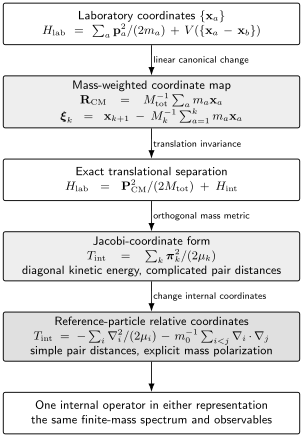
Coordinate choices redistribute algebra without changing the internal physics. Mass-weighted Jacobi vectors diagonalize $T_{\mathrm{int}}$; reference-particle vectors simplify pair separations but expose finite-mass cross derivatives.

Factorization of translational motion

For a total-momentum generalized eigenstate, the laboratory wavefunction can be written

$$\Psi_{\mathbf P} \left( \mathbf R_{\mathrm{CM}},\xi \right) = \exp\!\left( \frac{i\mathbf P\cdot\mathbf R_{\mathrm{CM}}}{\hbar} \right) \psi_{\mathrm{int}}(\xi),$$

with energy

$$E_{\mathrm{lab}} = \frac{P^2}{2M_{\mathrm{tot}}} + E_{\mathrm{int}}.$$

The plane wave is not square-integrable on all space; it has the usual continuum normalization. A localized molecular beam is a wavepacket in $\mathbf P$. Internal bound states can be normalizable even though the full free-molecule spectrum is continuous because of overall translation.

Reduced Mass and Mass Polarization

Jacobi coordinates are not always the most intuitive. Choose one particle, labeled $0$, as a reference and define

$$\mathbf x_i = \mathbf X_i-\mathbf X_0, \qquad i=1,\ldots,K-1.$$

After the center of mass is removed, the internal Hamiltonian takes the form

$$\begin{aligned} H_{\mathrm{int}} ={}& -\sum_{i=1}^{K-1} \frac{\hbar^2}{2\mu_i} \nabla_{\mathbf x_i}^2 \\ &- \frac{\hbar^2}{m_0} \sum_{i<j} \nabla_{\mathbf x_i} \mathbin{\cdot} \nabla_{\mathbf x_j} + V(\{\mathbf x_i\}), \end{aligned}$$

where

$$\mu_i = \frac{m_0m_i}{m_0+m_i}.$$

The cross-derivative term is called a mass-polarization, recoil, or specific-mass term, depending on context. It records the fact that motion of several particles relative to the same finite-mass reference cannot be independent.

Two warnings are important:

• reduced masses and the cross term are both finite-mass effects;
• mass polarization is coordinate-generated kinetic coupling, not an extra force.

In the formal limit $m_0\to\infty$,

$$\mu_i\to m_i, \qquad \frac{1}{m_0}\to0,$$

so the reference particle becomes immobile and the cross derivatives vanish.

Why the cross term appears

In the center-of-mass frame,

$$\mathbf p_0 = -\sum_{i=1}^{K-1}\mathbf p_i.$$

Hence the reference-particle kinetic energy contributes

$$\frac{\mathbf p_0^2}{2m_0} = \frac{1}{2m_0} \left( \sum_i\mathbf p_i \right)^2.$$

Expanding the square gives

$$\frac{\mathbf p_0^2}{2m_0} = \sum_i\frac{\mathbf p_i^2}{2m_0} + \frac{1}{m_0} \sum_{i<j} \mathbf p_i\mathbin{\cdot}\mathbf p_j.$$

The diagonal pieces combine with $\mathbf p_i^2/(2m_i)$ to produce $\mu_i$; the off-diagonal pieces become the cross gradients.

Two particles as the clean limit

For two particles there is one internal vector

$$\mathbf r=\mathbf x_2-\mathbf x_1$$

and no cross term. The exact separation is

$$H = \frac{\mathbf P_{\mathrm{CM}}^2}{2M} + \frac{\mathbf p^2}{2\mu} + V(r),$$

where

$$M=m_1+m_2, \qquad \mu=\frac{m_1m_2}{m_1+m_2}.$$

The reduced mass is therefore not a Born–Oppenheimer correction. It is the exact internal mass for a two-body translation-invariant problem.

Diatomic Internal Coordinates

For nuclei $A$ and $B$, the internuclear vector

$$\mathbf R=\mathbf R_B-\mathbf R_A$$

is a natural internal coordinate, with bare nuclear reduced mass

$$\mu_N = \frac{M_AM_B}{M_A+M_B}.$$

The corresponding relative kinetic piece has the form

$$T_R = -\frac{\hbar^2}{2\mu_N} \nabla_{\mathbf R}^2.$$

This does not by itself separate nuclear motion from electronic motion. Electron coordinates must be defined relative to a compatible origin, and finite-mass cross terms depend on that choice. Decomposing $\nabla_{\mathbf R}^2$ into radial and angular parts is exact, but interpreting those pieces as an isolated vibrator and rigid rotor requires a potential-surface and body-fixed reduction.

The Clamped-Nuclei Electronic Hamiltonian

The standard electronic operator at a specified nuclear geometry $R$ is, in atomic units,

$$\begin{aligned} H_e(R) ={}& -\frac12\sum_i\nabla_i^2 -\sum_{i,A}\frac{Z_A}{r_{iA}} \\ &+ \sum_{i<j}\frac{1}{r_{ij}} + \sum_{A<B}\frac{Z_AZ_B}{R_{AB}}. \end{aligned}$$

It acts only on electronic variables:

$$H_e(R)\phi_\alpha(r;R) = E_\alpha(R)\phi_\alpha(r;R).$$

Here $R$ labels parameters rather than dynamical arguments of the electronic eigenfunction. The last term is therefore a geometry-dependent scalar.

An equally common convention defines

$$H_{\mathrm{el}}(R) = H_e(R)-V_{NN}(R)$$

and then forms the surface

$$U_\alpha(R) = \mathcal E_\alpha(R)+V_{NN}(R).$$

The two conventions yield the same $U_\alpha$ when used consistently.

What has changed

Passing from $H_{\mathrm{int}}$ to $H_e(R)$ is not merely removal of the center of mass. It additionally:

1. treats nuclear coordinates as parameters in an auxiliary eigenproblem;
2. omits nuclear kinetic action during that electronic diagonalization;
3. usually neglects finite-mass terms in the electronic operator at leading order;
4. restores nuclear quantum motion only in a subsequent channel or surface equation.

The exact electronic-channel expansion can still retain all surfaces and derivative couplings. The Born–Oppenheimer approximation begins when that coupled problem is truncated or its couplings are neglected. Born–Oppenheimer in Molecules follows this reduction through equilibrium structure, isotope-dependent nuclear motion, rovibrational states, and spectroscopic corrections.

Worked Hamiltonians

The hydrogen molecular ion

For $\mathrm H_2^+$ there are two protons and one electron. In atomic units, before center-of-mass removal,

$$\begin{aligned} H_{\mathrm H_2^+} ={}& -\frac12\nabla_{\mathbf r}^2 -\frac{1}{2M_p}\nabla_A^2 -\frac{1}{2M_p}\nabla_B^2 \\ &- \frac{1}{r_A} - \frac{1}{r_B} + \frac{1}{R}. \end{aligned}$$

At clamped internuclear separation $R$, place the nuclei at $\pm\mathbf R/2$. The electronic problem is

$$H_e(R) = -\frac12\nabla_{\mathbf r}^2 -\frac{1}{r_A} -\frac{1}{r_B} +\frac{1}{R}.$$

Solving this equation for many values of $R$ produces an electronic potential-energy curve. Quantized vibration and rotation are not yet included. H₂⁺ Ion owns the exact two-center structure, minimal LCAO solution, bonding interpretation, and comparison with accurate Born–Oppenheimer benchmarks.

The hydrogen molecule

For $\mathrm H_2$, two electrons add one electron–electron pair:

$$\begin{aligned} H_{\mathrm H_2} ={}& -\frac12 \left( \nabla_1^2+\nabla_2^2 \right) -\frac{1}{2M_p} \left( \nabla_A^2+\nabla_B^2 \right) \\ &- \sum_{i=1}^{2} \left( \frac{1}{r_{iA}}+\frac{1}{r_{iB}} \right) \\ &+ \frac{1}{r_{12}} +\frac{1}{R}. \end{aligned}$$

This four-particle operator already contains covalent binding, exchange symmetry, electron correlation, nuclear motion, and dissociation. A molecular-orbital or valence-bond wavefunction is an approximation to states of this operator or of a controlled reduction of it. Hydrogen Molecule carries the clamped-nuclei reduction into the canonical comparison of Heitler–London, restricted Hartree–Fock, and correlated dissociation.

High-precision calculations may solve the four-body nonrelativistic problem directly and then add relativistic, radiative, and finite-size corrections. That route is conceptually distinct from first constructing one potential-energy surface, though both can reach exceptional accuracy for light molecules when their correction ledgers are complete.

Energy Zeros and Dissociation Thresholds

Adding a constant to a Hamiltonian does not change dynamics, but molecular binding requires a common energy convention.

For a channel in which the system separates into fragments $F_1,\ldots,F_s$, define the threshold from fragment energies computed with:

• the same particle masses;
• the same relativistic or nonrelativistic model;
• the same external-field assumptions;
• compatible internal quantum numbers;
• the same energy zero.

Then a dissociation energy can be written

$$D = E_{\mathrm{threshold}} - E_{\mathrm{molecule}}.$$

A positive $D$ indicates binding relative to that channel. The “lowest threshold” must be understood within the conserved symmetry sector; a lower-energy fragmentation channel forbidden by exact quantum numbers does not automatically determine the decay width of the state under consideration.

At infinite separation, neutral fragments can have vanishing leading Coulomb interaction while retaining dispersion and multipolar tails. Ionic fragments can retain a $1/R$ Coulomb term. Therefore “set $V=0$ at infinity” is a convention that must be matched to the actual asymptotic channel.

Energy and Length Scales

Let

$$\mu=\frac{m_e}{M}$$

for a representative nuclear mass. Near a smooth, nondegenerate molecular minimum, it is useful to define

$$\kappa=\mu^{1/4}.$$

The Born–Oppenheimer hierarchy then has the schematic orders:

Sector	Typical order in electronic atomic units
Electronic structure	$E_{\mathrm{el}}\sim E_h$ and lengths $\sim a_0$
Nuclear displacement	$\Delta R/a_0\sim\kappa$ near a regular minimum
Vibrational spacing	$E_{\mathrm{vib}}/E_h\sim\kappa^2=\mu^{1/2}$
Rotational spacing	$E_{\mathrm{rot}}/E_h\sim\kappa^4=\mu$
Regular recoil terms	often proportional to one or more powers of $\mu$

These are ordering estimates, not universal numerical formulas. Force constants, equilibrium bond lengths, electronic gaps, symmetry, anharmonicity, and proximity to dissociation can alter coefficients or invalidate the regular expansion.

For a proton,

$$\frac{m_e}{M_p} \approx \frac{1}{1836},$$

so

$$\mu^{1/2}\approx2.3\times10^{-2}, \qquad \mu\approx5.4\times10^{-4}.$$

This explains why vibrational spacings are often much smaller than electronic spacings and rotational spacings smaller still. It does not prove that one electronic surface is adequate: small electronic gaps can overwhelm the mass hierarchy.

Approximation Ledger

The nonrelativistic Coulomb Hamiltonian is a highly successful leading model, not an exact theory of nature.

Point nuclei

Nuclei are treated as structureless point charges with specified masses and spins. Finite charge radii, electric quadrupole moments, magnetic moments, polarizabilities, and internal nuclear excitation are omitted.

Electrostatic interaction

The interaction is instantaneous Coulomb interaction. Magnetic retardation, transverse photons, and radiative self-energy are absent.

Nonrelativistic particles

The kinetic energy is $p^2/(2m)$. For higher precision or heavy elements, scalar-relativistic effects, spin–orbit coupling, Breit interactions, and a relativistic electronic framework may be required.

Fixed particle number

Ionization and dissociation can be represented as continuum channels with the same particles, but pair creation, annihilation, and photon emission require a field-theoretic description.

Isolated system

No substrate, solvent, collision partner, trap, thermal bath, or measurement apparatus is included. Adding an environment changes the Hamiltonian or requires an open-system reduction.

Spin-free leading operator

Electron and nuclear spins label symmetry sectors but do not affect the Coulomb energy directly. Fine, hyperfine, Zeeman, and spin-rotation structure require additional terms.

External Fields

For particles with charges $q_a$, minimal coupling replaces

$$\mathbf p_a \longrightarrow \mathbf p_a-q_a\mathbf A(\mathbf x_a,t)$$

and adds scalar-potential energy $q_a\Phi$. The kinetic term becomes

$$T = \sum_a \frac{ \left[ \mathbf p_a-q_a\mathbf A(\mathbf x_a,t) \right]^2 }{2m_a}.$$

Spin couplings must be added consistently when relevant.

An electric field varying negligibly across a neutral molecule can often be expressed through an internal multipole interaction after the center of mass is handled. A magnetic field is subtler because the vector potential depends on position and ordinary canonical momentum is gauge dependent. Center-of-mass and internal motion need not separate in the field-free way; conserved pseudomomentum and the total charge become important. Magnetic Translations develops the associated symmetry.

The field-free formula

$$H_{\mathrm{lab}} = \frac{P_{\mathrm{CM}}^2}{2M_{\mathrm{tot}}} +H_{\mathrm{int}}$$

should therefore not be imported unchanged into a charged molecule in a magnetic field.

Common Mistakes

Calling the laboratory Hamiltonian an internal Hamiltonian

If free center-of-mass kinetic energy is still present, computed eigenstates include an irrelevant translational continuum. State the coordinate frame and whether translation has been removed.

Setting nuclear kinetic energy to zero without naming an approximation

$T_N$ is part of the exact nonrelativistic problem. Its omission defines a fixed-geometry electronic reduction.

Treating nuclear repulsion as always constant

$V_{NN}$ is constant only inside a clamped-geometry electronic calculation. It is a coordinate-dependent operator in the all-particle problem.

Using both ordered and unordered pair sums

$\sum_{i<j}$ counts each pair once. $\frac12\sum_{i\ne j}$ is equivalent. Combining the factor $1/2$ with $i<j$ undercounts the interaction.

Replacing every electron mass by a reduced mass

For more than two particles, reduced masses alone are generally insufficient. Cross derivatives or an equivalent Jacobi-coordinate structure are needed.

Calling mass polarization a new interaction

It is a kinetic coupling produced by the internal coordinate choice. Different coordinate systems can hide or expose it while representing the same physics.

Assigning a point group to the exact free molecule

Point-group symmetry belongs to a selected geometry or effective structural description. The exact isolated Hamiltonian has translation, rotation, parity, and permutation symmetries.

Comparing energies from inconsistent models

A molecular energy including recoil and radiative corrections cannot be subtracted consistently from a fragment threshold lacking those terms.

Assuming heavy nuclei guarantee adiabaticity

The mass ratio supplies a small parameter, but electronic degeneracies and small gaps can make derivative couplings large.

A Reliable Construction Workflow

For a new molecular calculation:

1. List particles, isotopes, charges, masses, and spin species.
2. Declare SI or atomic units and the energy zero.
3. Write all five Coulomb-Hamiltonian contributions.
4. Identify exact translation, rotation, parity, time-reversal, and permutation symmetries.
5. Remove overall translation with an explicit coordinate convention.
6. Record every reduced-mass and cross-derivative term.
7. Specify the approximation hierarchy: all-particle, coupled surfaces, one surface, rigid rotor, harmonic vibration, or another effective model.
8. Define observables and thresholds within the same Hamiltonian ledger.
9. Add relativistic, radiative, nuclear, environmental, or field terms only to the accuracy required.
10. Test coordinate invariance, limiting masses, dissociation limits, and exchange symmetry.

Exercises

Exercise 1: Recover atomic units

Starting from the SI electron kinetic and electron–nuclear terms, rescale lengths by $a_0$ and energies by $E_h$. Show that their coefficients become $-1/2$ and $-Z_A$, respectively.

Solution

Write

$$\mathbf r=a_0\boldsymbol\rho, \qquad \nabla_{\mathbf r} = \frac{1}{a_0}\nabla_{\boldsymbol\rho}.$$

Using

$$a_0 = \frac{4\pi\epsilon_0\hbar^2}{m_ee^2}$$

and

$$E_h = \frac{\hbar^2}{m_ea_0^2} = \frac{e^2}{4\pi\epsilon_0a_0},$$

the kinetic term becomes

$$-\frac{\hbar^2}{2m_ea_0^2} \nabla_{\boldsymbol\rho}^2 = -\frac{E_h}{2} \nabla_{\boldsymbol\rho}^2.$$

The attraction becomes

$$-\frac{Z_Ae^2} {4\pi\epsilon_0a_0\rho} = -E_h\frac{Z_A}{\rho}.$$

Dividing the Hamiltonian by $E_h$ gives the atomic-unit coefficients.

Exercise 2: Verify translation invariance

Show directly that translating every particle by the same vector $\mathbf a$ leaves the Coulomb potential unchanged. Explain why translating electrons but not nuclei is not a symmetry.

Solution

Under a common translation,

$$\mathbf x_a\longrightarrow\mathbf x_a+\mathbf a.$$

Every pair difference obeys

$$(\mathbf x_a+\mathbf a) - (\mathbf x_b+\mathbf a) = \mathbf x_a-\mathbf x_b.$$

All Coulomb denominators and the kinetic operator are therefore unchanged. If only electrons are translated, then

$$\mathbf r_i-\mathbf R_A \longrightarrow \mathbf r_i-\mathbf R_A+\mathbf a,$$

so $V_{eN}$ changes. The symmetry moves the entire isolated system, not one subsystem relative to another.

Exercise 3: Three-particle Jacobi masses

For masses $m_1,m_2,m_3$, choose

$$\boldsymbol\xi_1 = \mathbf x_2-\mathbf x_1$$

and

$$\boldsymbol\xi_2 = \mathbf x_3 - \frac{m_1\mathbf x_1+m_2\mathbf x_2} {m_1+m_2}.$$

Find the two Jacobi reduced masses.

Solution

The first coordinate measures particle $2$ relative to particle $1$, so

$$\mu_1 = \frac{m_1m_2}{m_1+m_2}.$$

The second measures particle $3$ relative to a cluster of mass $m_1+m_2$, so

$$\mu_2 = \frac{m_3(m_1+m_2)} {m_1+m_2+m_3}.$$

Together with $\mathbf R_{\mathrm{CM}}$, these coordinates diagonalize the free kinetic energy:

$$T = \frac{\mathbf P_{\mathrm{CM}}^2} {2(m_1+m_2+m_3)} + \frac{\boldsymbol\pi_1^2}{2\mu_1} + \frac{\boldsymbol\pi_2^2}{2\mu_2}.$$

Exercise 4: Derive mass polarization

Use a finite-mass reference particle $0$ and two relative momenta $\mathbf p_1,\mathbf p_2$. In the center-of-mass frame, derive the cross term in the internal kinetic energy.

Solution

The center-of-mass condition gives

$$\mathbf p_0 = -\mathbf p_1-\mathbf p_2.$$

Therefore

$$\begin{aligned} T ={}& \frac{(\mathbf p_1+\mathbf p_2)^2}{2m_0} + \frac{\mathbf p_1^2}{2m_1} + \frac{\mathbf p_2^2}{2m_2} \\ ={}& \frac{\mathbf p_1^2}{2\mu_1} + \frac{\mathbf p_2^2}{2\mu_2} + \frac{\mathbf p_1\mathbin{\cdot}\mathbf p_2}{m_0}. \end{aligned}$$

With $\mathbf p_i=-i\hbar\nabla_i$, the last term is

$$-\frac{\hbar^2}{m_0} \nabla_1\mathbin{\cdot}\nabla_2.$$

It vanishes in the infinite-reference-mass limit.

Exercise 5: Audit the hydrogen molecular ion

For clamped $\mathrm H_2^+$, identify which terms in the full three-particle Hamiltonian disappear from the electronic eigenproblem and which nuclear term remains as a scalar.

Solution

Both proton kinetic terms are omitted while solving the fixed-$R$ electronic problem:

$$-\frac{1}{2M_p}\nabla_A^2 -\frac{1}{2M_p}\nabla_B^2 \longrightarrow0.$$

The electron kinetic energy and both electron–proton attractions remain. The proton–proton repulsion

$$\frac{1}{R}$$

remains if the convention includes $V_{NN}$ in $H_e(R)$, but it is now a scalar parameter rather than a nuclear-coordinate operator. Nuclear quantum motion must be restored in a later equation.

Exercise 6: Point group or exact symmetry?

A bent triatomic molecule has a clamped equilibrium geometry with point group $C_{2v}$. Is $C_{2v}$ the complete exact symmetry of the freely translating and rotating all-particle Hamiltonian? Explain.

Solution

No. $C_{2v}$ classifies an electronic or rovibrational reduction relative to the selected geometry. The all-particle field-free Coulomb Hamiltonian is invariant under continuous common translations and rotations, parity, time reversal, and permutations of identical particles. A freely rotating stationary state is not fixed at one laboratory orientation. The point group remains extremely useful, but it is a reduced structural symmetry rather than the complete exact group.

Exercise 7: Isotope scaling

In the leading smooth-minimum hierarchy, estimate how vibrational and rotational spacings change when a characteristic nuclear mass doubles while the electronic surface is held fixed.

Solution

The schematic scalings are

$$E_{\mathrm{vib}}\propto M^{-1/2}, \qquad E_{\mathrm{rot}}\propto M^{-1}.$$

Thus

$$\frac{E_{\mathrm{vib}}(2M)} {E_{\mathrm{vib}}(M)} = \frac{1}{\sqrt2},$$

and

$$\frac{E_{\mathrm{rot}}(2M)} {E_{\mathrm{rot}}(M)} = \frac12.$$

Real isotopic shifts also contain adiabatic, nonadiabatic, geometric, and small nuclear-size effects, so this is the leading fixed-surface estimate.

Exercise 8: Consistent dissociation energy

Suppose a molecular energy includes finite nuclear mass but its separated-atom threshold was computed with infinitely heavy nuclei. Why is their difference not a controlled dissociation energy?

Solution

The two numbers are eigenvalues of different Hamiltonians. Their difference contains the desired binding energy plus an unmatched recoil contribution. One must compute molecule and fragments with the same isotope masses and correction ledger, then subtract:

$$D = E_{\mathrm{fragments}}^{\mathrm{same\ model}} - E_{\mathrm{molecule}}^{\mathrm{same\ model}}.$$

The same consistency requirement applies to relativistic, radiative, field, and finite-size corrections.

Summary

• The standard molecular Hamiltonian contains electron and nuclear kinetic energies plus all three Coulomb pair sectors.
• Overall translation separates exactly for an isolated field-free system.
• Internal coordinates can diagonalize the kinetic energy or expose reduced-mass and mass-polarization terms; these are equivalent representations.
• Electron antisymmetry and identical-nucleus statistics are part of the state space, not optional corrections.
• The clamped-nuclei electronic Hamiltonian is an auxiliary geometry-parameterized operator used in a later scale-separation scheme.
• Molecular binding is defined relative to a consistently modeled fragmentation threshold.
• Relativity, QED, nuclear structure, environments, and external fields lie outside the leading Coulomb model and must be added deliberately.

Connections

• Molecular Quantum Mechanics
• Common Molecular Hamiltonians
• Born–Oppenheimer Approximation as Scale Separation
• Born–Oppenheimer in Molecules
• Nonadiabatic Coupling
• Conical Intersections
• Potential Energy Surfaces
• Rotations of Molecules
• Vibrations of Diatomics
• Normal Modes of Polyatomics
• Rovibrational Coupling
• Electronic Structure Overview
• Atomic Units and Scales
• Exchange and Correlation
• Translation-Invariant Hamiltonians
• Fermions
• Parity
• Magnetic Translations
• Quantum Chemistry Roadmap
• Quantum Chemistry References

References

1. M. Born and R. Oppenheimer, “Zur Quantentheorie der Molekeln,” Annalen der Physik 389, 457–484 (1927), doi:10.1002/andp.19273892002.
2. M. Born and K. Huang, Dynamical Theory of Crystal Lattices (Clarendon Press, 1954), Chapters IV–V.
3. B. T. Sutcliffe, “Coordinate Systems and Transformations,” in S. Wilson, ed., Handbook of Molecular Physics and Quantum Chemistry, Vol. 1 (Wiley, 2003), pp. 485–500.
4. B. T. Sutcliffe, “Molecular Hamiltonians,” in S. Wilson, ed., Handbook of Molecular Physics and Quantum Chemistry, Vol. 1 (Wiley, 2003), pp. 501–525.
5. B. T. Sutcliffe and R. G. Woolley, “Molecular Structure Calculations without Clamping the Nuclei,” Physical Chemistry Chemical Physics 7, 3664–3676 (2005), doi:10.1039/B509723C.
6. B. T. Sutcliffe and R. G. Woolley, “On the Quantum Theory of Molecules,” Journal of Chemical Physics 137, 22A544 (2012), doi:10.1063/1.4755287.
7. E. Mátyus, “Pre-Born–Oppenheimer Molecular Structure Theory,” Molecular Physics 117, 590–609 (2019), doi:10.1080/00268976.2018.1530461.
8. M. Cafiero, S. Bubin, and L. Adamowicz, “Non-Born–Oppenheimer Calculations of Atoms and Molecules,” Physical Chemistry Chemical Physics 5, 1491–1501 (2003), doi:10.1039/B211193D.
9. S. Bubin, M. Pavanello, W.-C. Tung, K. L. Sharkey, and L. Adamowicz, “Born–Oppenheimer and Non-Born–Oppenheimer, Atomic and Molecular Calculations with Explicitly Correlated Gaussians,” Chemical Reviews 113, 36–79 (2013), doi:10.1021/cr200419d.
10. K. Pachucki and J. Komasa, “Nonadiabatic Rotational States of the Hydrogen Molecule,” Physical Chemistry Chemical Physics 20, 247–255 (2018), doi:10.1039/C7CP06516G.
11. J. Komasa, M. Puchalski, P. Czachorowski, G. Łach, and K. Pachucki, “Rovibrational Energy Levels of the Hydrogen Molecule through Nonadiabatic Perturbation Theory,” Physical Review A 100, 032519 (2019), doi:10.1103/PhysRevA.100.032519.
12. T. Kato, “Fundamental Properties of Hamiltonian Operators of Schrödinger Type,” Transactions of the American Mathematical Society 70, 195–211 (1951), doi:10.1090/S0002-9947-1951-0041010-X.
13. T. Kato, “On the Eigenfunctions of Many-Particle Systems in Quantum Mechanics,” Communications on Pure and Applied Mathematics 10, 151–177 (1957), doi:10.1002/cpa.3160100201.
14. W. Hunziker and I. M. Sigal, “The Quantum N-Body Problem,” Journal of Mathematical Physics 41, 3448–3510 (2000), doi:10.1063/1.533319.
15. J. E. Avron, I. W. Herbst, and B. Simon, “Separation of Center of Mass in Homogeneous Magnetic Fields,” Annals of Physics 114, 431–451 (1978), doi:10.1016/0003-4916(78)90276-2.
16. A. Abedi, N. T. Maitra, and E. K. U. Gross, “Exact Factorization of the Time-Dependent Electron-Nuclear Wave Function,” Physical Review Letters 105, 123002 (2010), doi:10.1103/PhysRevLett.105.123002.
17. T. Helgaker, P. Jørgensen, and J. Olsen, Molecular Electronic-Structure Theory (Wiley, 2000), Chapters 1 and 12.
18. P. R. Bunker and P. Jensen, Molecular Symmetry and Spectroscopy, 2nd ed. (NRC Research Press, 1998), Chapters 2–4.