Rovibrational Coupling

A rovibrational state carries rotational and vibrational quantum structure at the same time. The simplest approximation adds a rigid-rotor term to an independent harmonic or anharmonic vibration. A real molecule is not exactly separable: vibration changes the inertia tensor, rotation changes the effective nuclear potential, and Coriolis terms exchange angular momentum between overall and internal motion.

This coupling is visible directly in a resolved gas-phase infrared band. One vibrational transition becomes a family of rotational lines. Their positions form $P$, $Q$, and $R$ branches; their spacings determine rotational constants in two vibrational states; their intensities encode populations, angular line strengths, transition-moment variation, and nuclear-spin statistics.

Three distinctions keep the analysis honest:

• a branch label states a change in rotational angular momentum, not an intensity or a universal selection rule;
• a band origin is a difference of vibration-dependent term values, not necessarily an observed line;
• fitted constants belong to an effective Hamiltonian and a declared vibrational state, not automatically to one equilibrium geometry.

Canonical Scope

This page is the canonical home for:

• the physical origin of rotation–vibration coupling in diatomic and polyatomic molecules;
• effective rovibrational term values and the Dunham organization;
• $P$, $Q$, and $R$ branch definitions and line-position formulas;
• vibrational dependence of rotational and centrifugal-distortion constants;
• Coriolis coupling, vibrational angular momentum, and branch structure beyond a simple diatomic;
• Hönl–London and Herman–Wallis factors at an interpretive level;
• combination differences, branch heads, assignments, fitting, and uncertainty checks.

Rotations of Molecules owns inertia tensors, rotor classes, pure rotational spectra, centrifugal distortion, and rotational fitting conventions. Vibrations of Diatomics owns one-dimensional vibrational potentials, term values, isotope scaling, anharmonicity, and dipole functions. Normal Modes of Polyatomics owns the polyatomic Hessian, normal coordinates, and first-order infrared and Raman activity. This page begins when rotation and vibration must be treated together.

Notation and Conventions

Spectroscopic formulas are compact only after the conventions are fixed:

• A double prime labels the lower state and a single prime labels the upper state: $v'',J''\to v',J'$.
• $J$ denotes total angular momentum excluding nuclear spin in the simple closed-shell examples.
• $G(v)$ is a vibrational term value and $F_v(J)$ a rotational term value, both in wavenumber units.
• Tildes on $\widetilde B_v$, $\widetilde D_v$, and $\widetilde\nu$ emphasize quantities in $\mathrm{cm}^{-1}$.
• $P$, $Q$, and $R$ mean $\Delta J=-1,0,+1$, respectively, with $\Delta J=J'-J''$.
• A line label such as $R(J'')$ uses the lower-state rotational quantum number.

When a source writes $B_v$ in hertz or energy units, factors of $h$ and $c$ differ from the formulas below. Compare dimensions before comparing numbers.

Separating Rotation and Vibration

Zeroth-order product model

Near one equilibrium geometry, a first approximation is

$$\hat H_0 = \hat H_{\mathrm{vib}} + \hat H_{\mathrm{rot}}.$$

For a closed-shell diatomic,

$$\hat H_{\mathrm{rot}} \approx \frac{\hat{\mathbf J}^2} {2I_e}, \qquad I_e=\mu R_e^2.$$

The product states

$$\lvert v,J,M\rangle_0 = \lvert v\rangle \otimes \lvert J,M\rangle$$

then have additive energies. This is a controlled organizing limit when rotational spacings are small compared with vibrational spacings and the bond-length distribution is narrow. It is not an exact factorization of the nuclear Hamiltonian.

The exact diatomic radial problem already couples them

On one electronic potential $U(R)$, the reduced radial equation at fixed $J$ is

$$\begin{aligned} \Bigg[ &- \frac{\hbar^2}{2\mu} \frac{d^2}{dR^2} + U(R) \\ &+ \frac{\hbar^2J(J+1)} {2\mu R^2} \Bigg] u_{vJ}(R) = E_{vJ}u_{vJ}(R). \end{aligned}$$

The centrifugal contribution depends on the same coordinate that vibrates. Define

$$U_{\mathrm{eff},J}(R) = U(R) + \frac{\hbar^2J(J+1)} {2\mu R^2}.$$

Increasing $J$ tilts the effective well toward larger $R$, changes its curvature, and eventually lowers the effective dissociation barrier. Thus the radial wavefunction is really $u_{vJ}$ rather than one $u_v$ shared by every $J$.

With $q=R-R_e$,

$$\frac{1}{R^2} = \frac{1}{R_e^2} \left[ 1 - 2\frac{q}{R_e} + 3\frac{q^2}{R_e^2} - \cdots \right].$$

The constant term gives the equilibrium rigid rotor. The terms proportional to $qJ(J+1)$, $q^2J(J+1)$, and higher powers are explicit rotation–vibration interactions.

Polyatomic form

For a semirigid polyatomic molecule in a molecule-fixed frame, define

$$\hat{\mathcal J}_\alpha \equiv \hat J_\alpha-\hat\pi_\alpha.$$

The rovibrational Hamiltonian then has the schematic structure

$$\begin{aligned} \hat H_{\mathrm{rv}} &= \hat H_{\mathrm{vib}} + \hat T_{\mathrm{rot}}(\mathbf q) + \hat V_{\mathrm{ord}}(\mathbf q), \\ \hat T_{\mathrm{rot}}(\mathbf q) &= \frac12 \sum_{\alpha,\beta} \mu_{\alpha\beta}(\mathbf q) \hat{\mathcal J}_\alpha \hat{\mathcal J}_\beta. \end{aligned}$$

Here:

• $\mu_{\alpha\beta}(\mathbf q)$ is a coordinate-dependent inverse inertia tensor;
• $\hat{\boldsymbol\pi}$ is vibrational angular momentum generated by internal motion;
• $\hat V_{\mathrm{ord}}$ represents operator-ordering or pseudopotential terms whose exact form depends on coordinates and convention.

An Eckart frame makes translation and rotation locally orthogonal to infinitesimal vibration at the reference geometry and suppresses avoidable first-order kinematic coupling. It does not remove genuine Coriolis coupling or the coordinate dependence of the inertia tensor.

Effective Rovibrational Term Values

Additive notation with state-dependent constants

For a simple diatomic state, write

$$\frac{E_{vJ}}{hc} = T(v,J) \approx G(v)+F_v(J).$$

A standard vibrational expansion is

$$\begin{aligned} G(v) ={}& \omega_e \left( v+\frac12 \right) \\ &- \omega_ex_e \left( v+\frac12 \right)^2 \\ &+ \omega_ey_e \left( v+\frac12 \right)^3 + \cdots. \end{aligned}$$

Let

$$X=J(J+1).$$

The corresponding semirigid rotational expansion is

$$F_v(J) = \widetilde B_vX - \widetilde D_vX^2 + \widetilde H_vX^3 + \cdots.$$

The constants depend on $v$. The notation is additive, but the dependence of $F_v$ on the vibrational state already records coupling.

Dunham organization

A more unified expansion is

$$T(v,J) = \sum_{k,l\ge0} Y_{kl} \left( v+\frac12 \right)^k \left[ J(J+1) \right]^l.$$

Leading correspondences are

$$\begin{aligned} Y_{10}&\approx\omega_e, & Y_{20}&\approx-\omega_ex_e, \\ Y_{01}&\approx\widetilde B_e, & Y_{11}&\approx-\alpha_e, \\ Y_{02}&\approx-\widetilde D_e. \end{aligned}$$

The mixed coefficients with $k>0$ and $l>0$ are rotation–vibration terms. The correspondences are approximate because alternative spectroscopic constants may absorb higher-order contributions differently.

The Dunham series is an effective local expansion, not a globally convergent representation up to dissociation. Its fitted coefficients are correlated, and the number of retained terms must be justified by the measured range and uncertainty.

Rotational Constants Depend on Vibrational State

Diatomic vibrational averaging

If the centrifugal term is averaged over a vibrational state before higher couplings are included, the wavenumber rotational constant is

$$\widetilde B_v = \frac{h} {8\pi^2c\mu} \left\langle v \left| \frac{1}{R^2} \right| v \right\rangle.$$

A common low-order parameterization uses

$$\xi_v=v+\frac12$$

and writes

$$\widetilde B_v = \widetilde B_e - \alpha_e\xi_v + \gamma_e\xi_v^2 + \cdots.$$

For many diatomics, $\alpha_e>0$: higher vibrational states sample larger mean separations, so $\widetilde B_v$ decreases. This is not merely the replacement $R\mapsto\langle R\rangle$. The constant averages $R^{-2}$, and both displacement and variance contribute.

One may define an effective distance

$$r_v^{\mathrm{eff}} = \sqrt{ \frac{h} {8\pi^2c\mu\widetilde B_v} }.$$

It is a distance inferred from a state-averaged rotational constant, not automatically the equilibrium distance $R_e$ or the expectation value $\langle R\rangle_v$.

Polyatomic constants

For a polyatomic molecule, each principal rotational constant changes with all occupied normal modes. A common semirigid expansion is

$$\begin{aligned} \widetilde A_{\mathbf v} &= \widetilde A_e - \sum_i \alpha_i^{A} \left( v_i+\frac{d_i}{2} \right) + \cdots, \\ \widetilde B_{\mathbf v} &= \widetilde B_e - \sum_i \alpha_i^{B} \left( v_i+\frac{d_i}{2} \right) + \cdots, \\ \widetilde C_{\mathbf v} &= \widetilde C_e - \sum_i \alpha_i^{C} \left( v_i+\frac{d_i}{2} \right) + \cdots. \end{aligned}$$

Here $d_i$ is the mode degeneracy. The constants $\alpha_i^A,\alpha_i^B,\alpha_i^C$ combine vibrational averaging, anharmonicity, and coordinate conventions. Their signs need not all match.

P, Q, and R Branches

Master line-position equation

For absorption from $(v'',J'')$ to $(v',J')$,

$$\begin{aligned} \widetilde\nu_{\mathrm{line}} ={}& \frac{ E_{v'J'}-E_{v''J''} } {hc} \\ ={}& \widetilde\nu_0 + F_{v'}(J') - F_{v''}(J''), \end{aligned}$$

where the band origin is

$$\widetilde\nu_0 = G(v')-G(v'').$$

The rotational branches are:

• $P$ branch: $J'=J''-1$, so $\Delta J=-1$.
• $Q$ branch: $J'=J''$, so $\Delta J=0$.
• $R$ branch: $J'=J''+1$, so $\Delta J=+1$.

These names classify line families after the relevant transition operator and state symmetries have decided which families are allowed.

The simplest parallel diatomic band

For an electric-dipole transition within a closed-shell $^1\Sigma$ electronic state,

$$\Delta J=\pm1.$$

The $P$ and $R$ branches occur, while the $Q$ branch is absent. One angular factor is

$$\begin{pmatrix} J'&1&J''\\ 0&0&0 \end{pmatrix}.$$

For $J'=J''$, the sum of the three angular momenta is $2J''+1$, which is odd, so this three-j symbol vanishes. The missing $Q$ branch is therefore a transition-matrix-element result, not a gap inserted into the energy spectrum.

If centrifugal distortion is neglected and the two vibrational states share one constant $\widetilde B$, then

$$\begin{aligned} \widetilde\nu_P(J'') &= \widetilde\nu_0 - 2\widetilde B J'', \qquad J''\ge1, \\ \widetilde\nu_R(J'') &= \widetilde\nu_0 + 2\widetilde B(J''+1), \qquad J''\ge0. \end{aligned}$$

The lines are separated by approximately $2\widetilde B$ within each branch. No line occurs at $\widetilde\nu_0$ in this model.

Different upper- and lower-state constants

Set

$$\widetilde B' = \widetilde B_{v'}, \qquad \widetilde B'' = \widetilde B_{v''}.$$

Then

$$\begin{aligned} \widetilde\nu_P(J'') ={}& \widetilde\nu_0 - \left( \widetilde B'+\widetilde B'' \right)J'' \\ &+ \left( \widetilde B'-\widetilde B'' \right)J''^2, \\[4pt] \widetilde\nu_R(J'') ={}& \widetilde\nu_0 + \left( \widetilde B'+\widetilde B'' \right)(J''+1) \\ &+ \left( \widetilde B'-\widetilde B'' \right)(J''+1)^2. \end{aligned}$$

Introduce the branch index

$$m = \begin{cases} -J'', & P\text{ branch},\\ J''+1, & R\text{ branch}. \end{cases}$$

Define

$$\begin{aligned} \Sigma_B &= \widetilde B'+\widetilde B'', \\ \Delta_B &= \widetilde B'-\widetilde B''. \end{aligned}$$

Both branches then obey the Fortrat form

$$\widetilde\nu(m) = \widetilde\nu_0 + \Sigma_Bm + \Delta_Bm^2,$$

with no $m=0$ transition in the simple $^1\Sigma$ band.

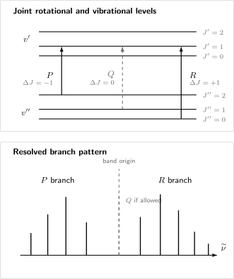
Rovibrational branch logic. The upper and lower vibrational manifolds each contain rotational levels. $P$, $Q$, and $R$ connect $\Delta J=-1,0,+1$; the $Q$ arrow and central stick are shown dashed because that branch is absent for a simple $^1\Sigma\leftrightarrow{}^1\Sigma$ parallel band but allowed in other symmetry and angular-momentum cases.

When a Q branch appears

A $Q$ branch can occur when the rovibrational angular factors and parity rules permit $\Delta J=0$. Examples include:

• perpendicular bands of linear polyatomic molecules;
• transitions involving nonzero electronic angular-momentum projection;
• degenerate vibrations carrying vibrational angular momentum;
• suitable symmetric-top parallel or perpendicular subbands with nonzero projection quantum numbers.

For a linear degenerate bend, the vibrational angular momentum quantum number $\ell$ supplies an internal projection absent from a nondegenerate diatomic stretch. A compact central $Q$ branch can then be one of the most prominent features of the band.

For symmetric and asymmetric tops, $P/Q/R$ labels classify only $\Delta J$. Each branch can contain many $K$-structured subbranches, asymmetry splittings, and parity components. A three-letter label may be needed to specify changes in projection quantum numbers and $J$.

Coriolis Coupling and Vibrational Angular Momentum

Degenerate vibrations can carry angular momentum about a molecular axis. Define dimensionless angular-momentum operators

$$\hat{\mathbf j} = \frac{\hat{\mathbf J}}{\hbar}, \qquad \hat{\boldsymbol\ell} = \frac{\hat{\boldsymbol\pi}}{\hbar}.$$

In a normal-coordinate basis, the leading Coriolis interaction in wavenumber units is schematically

$$\frac{\hat H_{\mathrm C}}{hc} \sim - 2 \sum_{\alpha,i,j} \widetilde B_\alpha \zeta_{ij}^{\alpha} \hat j_\alpha \hat\ell_{ij,\alpha},$$

up to convention-dependent tensor factors and symmetrization. The dimensionless coefficients $\zeta_{ij}^{\alpha}$ describe how vibrational motion transforms under rotation of the molecule-fixed frame.

Consequences include:

• splitting and mixing of levels within degenerate vibrational manifolds;
• $\ell$-type doubling in linear molecules;
• $K$-dependent shifts in symmetric tops;
• intensity borrowing between nominal bands;
• avoided crossings and assignment changes when levels of compatible symmetry approach.

For one degenerate bend of a linear molecule, a leading rotational term often contains

$$F_{v,\ell}(J) \approx \widetilde B_v \left[ J(J+1)-\ell^2 \right],$$

followed by Coriolis, $\ell$-doubling, and distortion corrections. The exact effective Hamiltonian and parity convention must be stated before comparing fitted constants.

Anharmonic and Centrifugal Corrections

Vibrational anharmonicity changes the band origin

For the fundamental $v''=0\to v'=1$,

$$\widetilde\nu_0 \approx \omega_e - 2\omega_ex_e + \cdots,$$

not simply $\omega_e$. Hot-band origins such as $1\to2$ are lower for the usual positive anharmonicity:

$$\widetilde\nu_{1\to2} \approx \omega_e - 4\omega_ex_e + \cdots.$$

Overtones and combination bands require both anharmonic term values and nonzero transition moments. Their rotational branches are built around their own band origins and vibrational-state constants.

Centrifugal distortion changes line spacings

Retaining the leading distortion term, let $X=J(J+1)$ and write

$$F_v(J) = \widetilde B_vX - \widetilde D_vX^2.$$

The negative term compresses the rotational ladder at high $J$. For a simple semirigid diatomic, the scale estimate

$$\widetilde D_e \sim \frac{ 4\widetilde B_e^3 }{ \omega_e^2 }$$

shows why distortion is usually much smaller than $\widetilde B_e$ but grows rapidly in importance with rotational excitation. This estimate is not a replacement for a fitted or calculated constant.

Upper and lower states generally have different $\widetilde D_v$. Their difference bends a Fortrat plot and shifts a predicted branch head. Higher constants $\widetilde H_v,\widetilde L_v,\ldots$ should be added only when residuals and measured range support them.

Resonances defeat isolated-band fits

Anharmonic, Coriolis, and centrifugal terms can bring two rovibrational basis states close in energy. If they have compatible exact symmetry, an effective block

$$\mathbf H_{\mathrm{eff}} = \begin{pmatrix} T_1(J) & W(J)\\ W(J)^* & T_2(J) \end{pmatrix}$$

produces avoided crossings and mixed eigenstates. Define

$$\begin{aligned} \overline T &= \frac{T_1+T_2}{2}, \\ \delta T &= \frac{T_1-T_2}{2}. \end{aligned}$$

The level shifts are then

$$T_\pm = \overline T \pm \sqrt{ \delta T^2 + |W|^2 }.$$

A high-order polynomial fitted through such a local perturbation may reproduce measured lines while predicting poorly outside them. Explicit coupled-state fitting is more interpretable when the interacting partner can be identified.

Rovibrational Line Intensities

Angular and vibrational factors

The space-fixed dipole component is obtained by rotating body-fixed components:

$$\mu_p^{\mathrm{SF}} = \sum_q D_{pq}^{1*}(\Omega) \mu_q^{\mathrm{BF}}(\mathbf q).$$

In the separable limit, a line strength factors into:

• a vibrational transition moment;
• a rotational Hönl–London factor;
• magnetic-sublevel and polarization sums;
• population and nuclear-spin statistical weights.

For a $^1\Sigma\leftrightarrow{}^1\Sigma$ band, one common unnormalized convention gives

$$S_P(J'')=J'', \qquad S_R(J'')=J''+1.$$

Their sum is $2J''+1$. Other tables normalize these factors differently, so an isolated Hönl–London number is incomplete without its convention.

Population envelope

At rotational temperature $T$, define $\beta=(k_{\mathrm B}T)^{-1}$. A simple lower-state population is

$$w_{J''} = g_{\mathrm{ns}}(J'') \left( 2J''+1 \right).$$

Then

$$N_{v''J''} \propto w_{J''} \exp \left[ -\beta hcF_{v''}(J'') \right].$$

Here $g_{\mathrm{ns}}$ is the nuclear-spin statistical weight. The observed integrated absorption also depends on transition frequency, stimulated-emission correction, line strength, column density, path length, line shape, optical depth, and instrumental response.

Alternating strong and weak lines can therefore reflect nuclear-spin statistics rather than alternating populations generated by the light source. Missing lines can reflect a selection rule, low population, blending, detector response, or inadequate sensitivity.

Herman–Wallis asymmetry

Exact rovibrational wavefunctions do not factor into one $J$-independent vibrational transition moment times a pure angular factor. Rotation changes the radial or normal-coordinate wavefunction and samples the coordinate dependence of the dipole moment.

For a diatomic band, this is often summarized by a Herman–Wallis factor

$$F_{\mathrm{HW}}(m) = \left( 1+A_1m+A_2m^2+\cdots \right)^2,$$

where $m<0$ labels $P$ lines and $m>0$ labels $R$ lines. The coefficients depend on the band, isotopologue, transition-moment expansion, and convention.

A nonzero odd coefficient makes corresponding $P$ and $R$ intensities asymmetric even after population and Hönl–London factors are removed. Treating every branch asymmetry as a temperature effect can therefore bias inferred populations.

Spectral Interpretation

Band origin, center, and maximum are different

The band origin $\widetilde\nu_0$ is the difference of vibrational term values at zero rotational contribution. A band center may mean a fitted origin, an intensity-weighted centroid, or a reported peak position. A band maximum depends on temperature, line strengths, broadening, and instrumental resolution.

In a simple $P/R$ band, no transition lies at the origin. In a band with a $Q$ branch, individual $Q(J)$ lines can still shift with $J$:

$$\widetilde\nu_Q(J) = \widetilde\nu_0 + \left( \widetilde B'-\widetilde B'' \right) J(J+1) + \cdots.$$

A sharp unresolved $Q$ feature is not automatically one line exactly at $\widetilde\nu_0$.

Combination differences

Combination differences eliminate one state and the band origin. Define the upper-state difference

$$\begin{aligned} \Delta_u(J) &\equiv \widetilde\nu_R(J)-\widetilde\nu_P(J), \\ &= F'(J+1)-F'(J-1). \end{aligned}$$

The lower-state difference is

$$\begin{aligned} \Delta_l(J) &\equiv \widetilde\nu_R(J-1) - \widetilde\nu_P(J+1), \\ &= F''(J+1)-F''(J-1). \end{aligned}$$

In the rigid-rotor limit,

$$\begin{aligned} \Delta_u(J) &= 2\widetilde B'(2J+1), \\ \Delta_l(J) &= 2\widetilde B''(2J+1). \end{aligned}$$

The first isolates upper-state spacings; the second isolates lower-state spacings. Combination differences are powerful assignment checks because calibration offsets and uncertain band origins cancel.

Branch heads

In the distortion-free Fortrat approximation,

$$\widetilde\nu(m) = \widetilde\nu_0 + \Sigma_Bm + \Delta_Bm^2,$$

where

$$\Sigma_B = \widetilde B'+\widetilde B'', \qquad \Delta_B = \widetilde B'-\widetilde B''.$$

Treating $m$ continuously gives a turning point at

$$m_{\mathrm{head}} = - \frac{\Sigma_B} {2\Delta_B}.$$

If $\widetilde B'<\widetilde B''$, then $\Delta_B<0$ and a positive-$m$ $R$-branch head can occur. If $\widetilde B'>\widetilde B''$, a negative-$m$ $P$-branch head is possible. The nearest allowed integer gives only a first estimate; centrifugal distortion, perturbations, population cutoff, and predissociation can move or erase the observed head.

A synthetic line pattern

Consider a hypothetical $^1\Sigma$ fundamental with

$$\begin{aligned} \widetilde\nu_0&=2000.00\,\mathrm{cm}^{-1}, \\ \widetilde B''&=1.90\,\mathrm{cm}^{-1}, \\ \widetilde B'&=1.87\,\mathrm{cm}^{-1}. \end{aligned}$$

Ignoring distortion,

$$\begin{aligned} \widetilde\nu_P(1) &= 1996.20\,\mathrm{cm}^{-1}, \\ \widetilde\nu_P(2) &= 1992.34\,\mathrm{cm}^{-1}, \\ \widetilde\nu_R(0) &= 2003.74\,\mathrm{cm}^{-1}, \\ \widetilde\nu_R(1) &= 2007.42\,\mathrm{cm}^{-1}. \end{aligned}$$

The gap around $2000.00\,\mathrm{cm}^{-1}$ identifies a missing simple-band $Q$ branch, while the slowly changing line spacings reveal $\widetilde B'\ne\widetilde B''$. These four lines do not by themselves justify high-order distortion or a global potential.

A defensible assignment workflow

1. State the isotopologue, electronic and vibrational states, pressure, temperature, calibration, resolution, and line-shape model.
2. Identify candidate branch direction from spacing trends, not from left/right position alone.
3. Apply parity, angular-momentum, and nuclear-spin selection rules.
4. Label lines with the lower-state quantum number and preserve prime conventions.
5. Form upper- and lower-state combination differences before a global fit.
6. Fit the lowest-order effective Hamiltonian supported by residuals and uncertainty.
7. Inspect residuals against $J$, branch, parity, isotopologue, and experimental subset.
8. Add distortion or explicit interacting states only when structured residuals require them.
9. Test intensities with populations, Hönl–London factors, and Herman–Wallis corrections separately.
10. Validate constants against pure rotational data, other vibrational bands, isotopologues, or independent calculations.

What the Spectrum Can and Cannot Determine

Resolved rovibrational lines can constrain:

• vibrational term differences and anharmonic intervals;
• upper- and lower-state rotational constants;
• centrifugal-distortion constants over the measured $J$ range;
• isotope-dependent inertia changes;
• Coriolis and resonance couplings;
• line-strength corrections and rotational temperatures;
• effective structures when enough isotopic and vibrational information is combined.

They do not determine uniquely:

• a global potential-energy surface from one band;
• an equilibrium geometry from one $\widetilde B_0$;
• a temperature from an uncorrected intensity envelope;
• a transition dipole from arbitrary-height plotted sticks;
• a high-$J$ extrapolation through an unmodeled resonance;
• a single “bond length during vibration” represented by the displayed mode arrows.

Common Mistakes

“Rotation and vibration are independent because the energies are added”

The effective sum $G(v)+F_v(J)$ already contains coupling through the $v$ dependence of $F_v$. The exact radial or polyatomic kinetic operator is not separable in that simple way.

“P, Q, and R are three universal allowed branches”

They are names for $\Delta J=-1,0,+1$. Symmetry, parity, angular-momentum projections, and the transition operator determine which branches have nonzero strength.

“The missing central line is the band origin”

The origin is a fitted term-value difference. In a simple $P/R$ band, there is no $m=0$ line at all.

“Every neighboring line has the same spacing”

That holds only when upper and lower rotational constants are equal and distortion is neglected. Real branch spacings vary with $J$.

“A branch head is a new energy level”

A branch head is a crowding and reversal of transition frequencies as the line index changes. It arises from differences between two rotational ladders.

“Relative line heights give a Boltzmann distribution directly”

Hönl–London factors, nuclear-spin weights, Herman–Wallis corrections, stimulated emission, optical depth, line shape, and instrument response also affect intensity.

“More fitted constants always improve the molecular model”

An over-parameterized effective Hamiltonian can interpolate noise and extrapolate badly. Parameter covariance and withheld-line prediction matter.

Exercises

1. Expose the coupling in the centrifugal term

Let $R=R_e+q$. Expand $R^{-2}$ through $q^2$ and identify the first two rotation–vibration coupling terms in

$$\frac{\hbar^2J(J+1)} {2\mu R^2}.$$

What qualitative displacement does the linear term favor for $J>0$?

Solution

Using

$$(1+x)^{-2} = 1-2x+3x^2+O(x^3),$$

one obtains

$$\frac{1}{R^2} = \frac{1}{R_e^2} \left[ 1 - 2\frac{q}{R_e} + 3\frac{q^2}{R_e^2} + O(q^3) \right].$$

Therefore

$$\begin{aligned} V_{\mathrm{cent}} ={}& \frac{\hbar^2J(J+1)} {2\mu R_e^2} \\ &- \frac{\hbar^2J(J+1)} {\mu R_e^3}q \\ &+ \frac{3\hbar^2J(J+1)} {2\mu R_e^4}q^2 + \cdots. \end{aligned}$$

The linear coefficient is negative, so increasing $q$ lowers the centrifugal contribution. Rotation therefore shifts the effective minimum toward larger separation: centrifugal stretching.

2. Derive the simple P and R formulas

Assume

$$F'(J)=F''(J)=\widetilde B J(J+1).$$

Derive the $P(J'')$ and $R(J'')$ line positions. Explain why $P(0)$ does not exist.

Solution

For the $P$ branch, $J'=J''-1$:

$$\begin{aligned} \widetilde\nu_P(J'') &= \widetilde\nu_0 + \widetilde B(J''-1)J'' \\ &\quad - \widetilde B J''(J''+1) \\ &= \widetilde\nu_0 - 2\widetilde B J''. \end{aligned}$$

For the $R$ branch, $J'=J''+1$:

$$\begin{aligned} \widetilde\nu_R(J'') &= \widetilde\nu_0 + \widetilde B(J''+1)(J''+2) \\ &\quad - \widetilde B J''(J''+1) \\ &= \widetilde\nu_0 + 2\widetilde B(J''+1). \end{aligned}$$

$P(0)$ would require $J'=-1$, which is not an angular-momentum quantum number. Thus the $P$ branch starts at $J''=1$, while the $R$ branch starts at $J''=0$.

3. Use combination differences

Show that, in the rigid-rotor approximation,

$$\widetilde\nu_R(J) - \widetilde\nu_P(J) = 2\widetilde B'(2J+1).$$

Why is this useful if the absolute wavenumber calibration has a constant offset?

Solution

Both lines start from the same lower level $J$:

$$\begin{aligned} \widetilde\nu_R(J) &= \widetilde\nu_0 + F'(J+1)-F''(J), \\ \widetilde\nu_P(J) &= \widetilde\nu_0 + F'(J-1)-F''(J). \end{aligned}$$

Subtracting cancels the lower term and origin:

$$\begin{aligned} F'(J+1) &= \widetilde B'(J+1)(J+2), \\ F'(J-1) &= \widetilde B'(J-1)J. \end{aligned}$$

Therefore

$$\widetilde\nu_R(J) - \widetilde\nu_P(J) = 2\widetilde B'(2J+1).$$

A constant calibration offset appears in both measured line positions and cancels in their difference. Nonlinear calibration error does not necessarily cancel.

4. Locate a branch head

For the synthetic constants

$$\widetilde B'=1.87\,\mathrm{cm}^{-1}, \qquad \widetilde B''=1.90\,\mathrm{cm}^{-1},$$

estimate the continuous Fortrat branch-head index and identify the branch.

Solution

Here

$$\begin{aligned} \Sigma_B &= 3.77\,\mathrm{cm}^{-1}, \\ \Delta_B &= -0.03\,\mathrm{cm}^{-1}. \end{aligned}$$

Therefore

$$m_{\mathrm{head}} = - \frac{3.77} {2(-0.03)} \approx 62.8.$$

Positive $m$ labels the $R$ branch, so the distortion-free model predicts an $R$-branch head near $m=63$, corresponding roughly to $J''=62$. At such high $J$, centrifugal distortion and population loss are likely important, so this is only a starting estimate.

5. Infer an effective distance ratio

For one isotopologue,

$$\widetilde B_0 = 1.900\,\mathrm{cm}^{-1}, \qquad \widetilde B_1 = 1.870\,\mathrm{cm}^{-1}.$$

Find $r_1^{\mathrm{eff}}/r_0^{\mathrm{eff}}$.

Solution

At fixed reduced mass,

$$r_v^{\mathrm{eff}} \propto \widetilde B_v^{-1/2}.$$

Thus

$$\frac{ r_1^{\mathrm{eff}} }{ r_0^{\mathrm{eff}} } = \sqrt{ \frac{ \widetilde B_0 }{ \widetilde B_1 } } = \sqrt{ \frac{1.900}{1.870} } \approx 1.0080.$$

The effective distance increases by about $0.80\%$. This ratio does not state that the molecule sits at one sharply defined radius in either vibrational state.

6. Diagnose the Q branch

Why is $\Delta J=0$ forbidden in the simple $^1\Sigma\leftrightarrow{}^1\Sigma$ electric-dipole band but possible for a degenerate bending band of a linear polyatomic molecule?

Solution

For the simple parallel $\Sigma$ band, both body-fixed projections are zero. The angular factor contains

$$\begin{pmatrix} J&1&J\\ 0&0&0 \end{pmatrix},$$

which vanishes because $J+1+J=2J+1$ is odd.

A degenerate bend carries nonzero vibrational angular momentum and has perpendicular transition-dipole components. The body-fixed projection quantum numbers in the three-j symbol are then not all zero, and the $\Delta J=0$ angular factor can be nonzero when parity and full symmetry also permit it. The label $Q$ says only $\Delta J=0$; the internal angular-momentum structure decides its strength.

7. Separate population from line strength

Two lines start from the same vibrational state and adjacent $J''$ values. The higher-$J''$ line is weaker. Give four reasons other than a lower Boltzmann population that could contribute.

Solution

Possible reasons include:

1. a smaller Hönl–London factor for that branch and quantum number;
2. a Herman–Wallis correction that suppresses that side of the band;
3. a different nuclear-spin statistical weight;
4. blending or unresolved hyperfine or parity structure;
5. optical-depth saturation of the comparison line;
6. a frequency-dependent source, detector, or instrument response;
7. pressure-dependent line-shape or baseline errors;
8. intensity borrowing or destructive mixing near a resonance.

Temperature inference requires a line-intensity model, not line heights alone.

8. Interpret structured residuals

A $P/R$ fit with $\widetilde B'$, $\widetilde B''$, $\widetilde D'$, and $\widetilde D''$ has random residuals except for a localized antisymmetric excursion around $J=18$ in both branches. What should be tested before adding still higher distortion constants?

Solution

A localized feature is more suggestive of a level interaction or assignment problem than of smooth centrifugal distortion. Test:

1. line blending, calibration, and the branch assignments near $J=18$;
2. parity or unresolved substructure;
3. combination differences to identify whether the perturbation lies in the upper or lower state;
4. nearby vibrational, electronic, or Coriolis-coupled states of compatible symmetry;
5. a small explicit coupled-state Hamiltonian with a physically motivated $W(J)$;
6. whether the feature repeats in another band sharing the perturbed state.

Adding high powers of $J(J+1)$ can hide the excursion while corrupting extrapolation.

Key Takeaways

• Rotation and vibration are only approximately separable because the inertia tensor and centrifugal potential depend on internal coordinates.
• Effective term values organize this coupling through vibrationally dependent rotational and distortion constants or mixed Dunham coefficients.
• $P$, $Q$, and $R$ label $\Delta J=-1,0,+1$; symmetry and the transition operator decide which branches are present.
• A simple $^1\Sigma$ parallel band has $P$ and $R$ branches but no $Q$ line at the band origin.
• Differences between upper- and lower-state constants curve branch spacings and can create a branch head.
• Combination differences isolate one rotational ladder and provide strong assignment checks.
• Coriolis coupling and vibrational angular momentum enrich polyatomic bands with $Q$ branches, splittings, mixing, and intensity borrowing.
• Line intensities require populations, Hönl–London factors, nuclear-spin weights, and rotation-dependent transition moments.
• A fitted rovibrational Hamiltonian has a declared range and convention; it should not be extrapolated blindly through resonances or toward dissociation.

Cross-Links

• Common Molecular Hamiltonians supplies the compact operator and unit dictionary that precedes a rovibrational fit.
• Molecular Quantum Mechanics places rovibrational coupling in the full molecular hierarchy.
• Molecular Hamiltonian gives the all-particle starting point and exact center-of-mass separation.
• Born–Oppenheimer in Molecules develops one-surface nuclear motion and nonadiabatic accuracy limits.
• Nonadiabatic Coupling separates weak effective-mass and level corrections from genuine multistate transfer and photochemical dynamics.
• Potential Energy Surfaces owns molecular curvature, stationary points, and global surface validity.
• Rotations of Molecules develops inertia tensors, rotor classes, pure rotational spectra, distortion, and fitting conventions.
• Vibrations of Diatomics develops vibrational potentials, term values, anharmonicity, isotope effects, and dipole functions.
• Normal Modes of Polyatomics develops collective vibrations, symmetry labels, and first-order infrared and Raman activity.
• Vibrational Spectroscopy develops the spectroscopy-facing assignment of band origins, hot bands, overtones, combinations, and anharmonic resonances.
• Infrared Spectroscopy applies rovibrational structure to gas-phase IR bands and separates transmission, ATR, and condensed-phase measurement models.
• Rigid Rotor gives the canonical angular eigenproblem.
• Rotational Spectra gives the first pure-rotational line ladder.
• Molecular Rotation Applications derives angular selection rules with tensor operators and three-j symbols.
• Selection Rules and Transition Rates separates symmetry zeros, operator choice, amplitudes, and rates.
• Molecular Physics maps molecular point-group, rotational, vibrational, and permutation symmetries.
• Quantum Chemistry Roadmap places molecular nuclear motion in a broader study sequence.
• Quantum Chemistry References provides a wider source ladder for molecular structure and spectroscopy.

References

• G. Herzberg, Molecular Spectra and Molecular Structure. I. Spectra of Diatomic Molecules, 2nd ed., Van Nostrand, 1950.
• G. Herzberg, Molecular Spectra and Molecular Structure. II. Infrared and Raman Spectra of Polyatomic Molecules, Van Nostrand, 1945.
• P. F. Bernath, Spectra of Atoms and Molecules, 4th ed., Oxford University Press, 2025.
• P. R. Bunker and P. Jensen, Molecular Symmetry and Spectroscopy, 2nd ed., NRC Research Press, 1998.
• J. M. Brown and A. Carrington, Rotational Spectroscopy of Diatomic Molecules, Cambridge University Press, 2003.
• D. Papoušek and M. R. Aliev, Molecular Vibrational-Rotational Spectra, Elsevier, 1982.
• E. B. Wilson Jr., J. C. Decius, and P. C. Cross, Molecular Vibrations: The Theory of Infrared and Raman Vibrational Spectra, McGraw–Hill, 1955; Dover reprint, 1980.
• J. L. Dunham, “The Energy Levels of a Rotating Vibrator,” Physical Review 41, 721–731 (1932), doi:10.1103/PhysRev.41.721.
• J. K. G. Watson, “Simplification of the Molecular Vibration-Rotation Hamiltonian,” Molecular Physics 15, 479–490 (1968), doi:10.1080/00268976800101381.
• H. Hönl and F. London, “Über die Intensitäten der Bandenlinien,” Zeitschrift für Physik 33, 803–809 (1925), doi:10.1007/BF01328367.
• R. C. Herman and R. F. Wallis, “Influence of Vibration–Rotation Interaction on Line Intensities in Vibration–Rotation Bands of Diatomic Molecules,” Journal of Chemical Physics 23, 637–646 (1955), doi:10.1063/1.1742069.
• J. K. G. Watson, “Hönl–London Factors for Multiplet Transitions in Hund’s Case a or b,” Journal of Molecular Spectroscopy 252, 5–8 (2008), doi:10.1016/j.jms.2008.04.014.
• NIST, Diatomic Spectral Database for $^1\Sigma$-Ground-State Molecules, definitions, Dunham coefficients, isotope scaling, and evaluated constants.
• IUPAC, “vibrational term value”, Compendium of Chemical Terminology, 5th ed., 2025, doi:10.1351/goldbook.08709.